第2章 局部图像描述子

引言

本章旨在寻找图像间的对应点和对应区域。

2.1 Harris角点检测器

Harris 角点检测算法（也称 Harris & Stephens 角点检测器）是一个极为简单的角点检测算法。该算法的主要思想是，如果像素周围显示存在多于一个方向的边，我们认为该点为兴趣点。该点就称为角点。

我们把图像域中点 x 上的对称半正定矩阵$M_I=M_I（x）$定义为：
$${\mathbf{M}}_I=\nabla \mathbf{I}\nabla {\mathbf{I}}^T=\left[\begin{array}{l}{\mathbf{I}}_x\\ {\mathbf{I}}_y\end{array}\right]\left[\begin{array}{ll}{\mathbf{I}}_x& {\mathbf{I}}_y\end{array}\right]=\left[\begin{array}{ll}{\mathbf{I}}_x^2& {\mathbf{I}}_x{\mathbf{I}}_y\\ {\mathbf{I}}_x{\mathbf{I}}_y& {\mathbf{I}}_y^2\end{array}\right]$$

其中$\nabla \mathbf{I}$为包含导数 $I_x$ 和$I_y$的图像梯度。由于该定义，$M_I$的秩为 1，特征值为${\lambda }_1=|\nabla I{|}^2\text{ 和 }{\lambda }_2=0$。

现在对于图像的每一个像素，我们可以计算出该矩阵。

选择权重矩阵 W（通常为高斯滤波器$G_{\sigma }$），我们可以得到卷积：
$${\overline{\mathbf{M}}}_I=\mathbf{W}\ast {\mathbf{M}}_I$$

该卷积的目的是得到$M_I$ 在周围像素上的局部平均。计算出的矩阵$M_I$ 又称为 Harris矩阵。W 的宽度决定了在像素 x 周围的感兴趣区域。像这样在区域附近对矩阵$M_I$取平均的原因是，特征值会依赖于局部图像特性而变化。如果图像的梯度在该区域变化，那么$M_I$的第二个特征值将不再为 0。如果图像的梯度没有变化，$M_I$的特征值也不会变化。

取决于该区域$I$的值， Harris 矩阵$M_I$的特征值有三种情况：

• 如果 λ1 和 λ2 都是很大的正数，则该 x 点为角点；
• 如果 λ1 很大， λ2 ≈ 0，则该区域内存在一个边，该区域内的平均$M_I$ 的特征值不会变化太大；
• 如果 λ1≈λ2≈0，该区域内为空。

在不需要实际计算特征值的情况下，为了把重要的情况和其他情况分开， Harris 和Stephens 引入了指示函数：
$$\det \left({\overline{\mathbf{M}}}_I\right)-\kappa \mathrm{trace}{\left({\overline{\mathbf{M}}}_I\right)}^2$$

为了去除加权常数 κ，我们通常使用商数：
$$\frac{\det \left({\bar{M}}_I\right)}{\mathrm{trace}{\left({\bar{M}}_I\right)}^2}$$

作为指示器。

from PIL import Image
from numpy import *
from pylab import *
from scipy.ndimage import filters
 
 

def harris_response(img, sigma):
    """ 函数功能：计算角点检测器的响应函数 
        参数说明：img__图像数据
                 sigma__高斯滤波参数
        函数返回：返回像素值为 Harris 响应函数值的一幅图像

    """
    # 导数计算
    img_x = zeros(img.shape)
    filters.gaussian_filter(img, (sigma, sigma), (0, 1), img_x)
    img_y = zeros(img.shape)
    filters.gaussian_filter(img, (sigma, sigma), (1, 0), img_y)
    # 计算Harris矩阵的分量,根据公式可以写出
    Wxx = filters.gaussian_filter(img_x*img_x, sigma)
    Wxy = filters.gaussian_filter(img_x*img_y, sigma)
    Wyy = filters.gaussian_filter(img_y*img_y, sigma)
    # 计算矩阵的特征值和迹
    Wdet = Wxx*Wyy - Wxy**2
    Wtr = Wxx + Wyy
    return Wdet / Wtr
 
 
def harris_points(harrisim, min_dist=10, threshold=0.1):
    """
    从一幅Harris响应图像中返回角点
    :param harrisim: 为harris_response响应得出的图像
    :param min_dist: 分割角点和图像边界的最少像素数目
    :param threshold: 阈值
    :return:
    """
    # 寻找高于阈值的候选角点
    corner_threshold = harrisim.max() * threshold
    harrisim_t = (harrisim > corner_threshold) * 1
 
    # 得到候选点的坐标(.T为转置)
    coords = array(harrisim_t.nonzero()).T
 
    # 以及它们的Harris响应值
    candidate_values = [harrisim[c[0], c[1]] for c in coords]
 
    # 对候选点按照harris响应值进行排序
    index = argsort(candidate_values)
 
    # 将可行点的位置保存到数组中
    allowed_locations = zeros(harrisim.shape)
    allowed_locations[min_dist:-min_dist, min_dist:-min_dist] = 1
 
    # 按照min_distance 原则，选择最佳Harris点
    filtered_coords = []
    for i in index:
        if allowed_locations[coords[i, 0], coords[i, 1]] == 1:
            filtered_coords.append(coords[i])
            allowed_locations[(coords[i, 0] - min_dist):(coords[i, 0] + min_dist),
            (coords[i, 1] - min_dist):(coords[i, 1] + min_dist)] = 0
    return filtered_coords

def cornerDetection(fileName):
    # 打开该图像，转换成灰度图像。
    img = array(Image.open(fileName).convert('L'))
    gray()
    # 计算响应函数，
    harrisim = harris_response(img, 10)
    # 基于响应值选择角点
    filtered_coords0 = harris_points(harrisim, 30, 0.01)
    filtered_coords1 = harris_points(harrisim, 30, 0.05)
    filtered_coords2 = harris_points(harrisim, 30, 0.1)

    # 在原始图像中覆盖绘制检测出的角点。
    subplot(231)
    imshow(img), title('original'),axis('off')  # 坐标轴隐去

    subplot(233)
    imshow(harrisim), title('harrisim'),axis('off')  

    subplot(234)
    imshow(img), title('thresholds = 0.01'),axis('off')
    plot([p[1] for p in filtered_coords0], [p[0] for p in filtered_coords0], "*")

    subplot(235)
    imshow(img), title('thresholds = 0.05'),axis('off')
    plot([p[1] for p in filtered_coords1], [p[0] for p in filtered_coords1], "*")

    subplot(236)
    imshow(img), title('thresholds = 0.1'),axis('off')
    plot([p[1] for p in filtered_coords2], [p[0] for p in filtered_coords2], "*")

    show()

    return


def main():
    fileName = r'D:\python\exercise_data\ComputerVision\ch02\\figure\empire.jpg'

    cornerDetection(fileName)

    return

if __name__ =="__main__":

    main()

输出结果如下：

图中右上的Harrisim函数为返回的像素值为 Harris 响应函数值的图像。选取像素值高于阈值的所有图像点；再加上额外的限制，即角点之间的间隔必须大于设定的最小距离获取所有的候选像素点，以角点响应值递减的顺序排序，然后将距离已标记为角点位置过近的区域从候选像素点中删除。

上图中下面一行对应的分别是将门限值设置为0.01、 0.05、0.1三个值。角点距离为30时，将检测到的角点图在原图上显示出来的。可以看到，阈值越小，检测到的角点越多。

在图像间寻找对应点

Harris 角点检测器仅仅能够检测出图像中的兴趣点，但是没有给出通过比较图像间的兴趣点来寻找匹配角点的方法。我们需要在每个点上加入描述子信息，并给出一个比较这些描述子的方法。

兴趣点描述子是分配给兴趣点的一个向量，描述该点附近的图像的表观信息。描述子越好，寻找到的对应点越好。我们用对应点或者点的对应来描述相同物体和场景点在不同图像上形成的像素点。

Harris 角点的描述子通常是由周围图像像素块的灰度值，以及用于比较的归一化互相关矩阵构成的。图像的像素块由以该像素点为中心的周围矩形部分图像构成。通常，两个（相同大小）像素块$I_1(x)$和$I_2(x)$的相关矩阵定义为：$$c\left({\mathbf{I}}_1,{\mathbf{I}}_2\right)=\sum f\left({\mathbf{I}}_1(\mathbf{x}),{\mathbf{I}}_2(\mathbf{x})\right)$$

函数 f 随着相关方法的变化而变化。上式取像素块中所有像素位置 x 的和。对于互相关矩阵，函数 $f(I_1，I_2)=I_1{I}_2$, 因此，$c(I_1，I_2)=I_1\cdot I_2$ , 其中 $\cdot$ 表示向量乘法（按照行或者列堆积的像素）。$c(I_1，I_2)$的值越大，像素块$I_1和I2$ 的相似度越高。

归一化的互相关矩阵是互相关矩阵的一种变形，可以定义为：
$$ncc\left({\mathbf{I}}_1,{\mathbf{I}}_2\right)=\frac{1}{n-1}\sum _{\mathbf{x}}\frac{\left({\mathbf{I}}_1(\mathbf{x})-{\mu }_1\right)}{{\sigma }_1}\cdot \frac{\left({\mathbf{I}}_2(\mathbf{x})-{\mu }_2\right)}{{\sigma }_2}$$

其中， n为像素块中像素的数目， μ1 和 μ2 表示每个像素块中的平均像素值强度， σ1和 σ2 分别表示每个像素块中的标准差。通过减去均值和除以标准差，该方法对图像亮度变化具有稳健性。

 
# 为获得图像像素块，并使用归一化的互相关矩阵来比较需要以下函数
def get_descriptor(image, filtered_coords, wid=5):
    """
    对于每个返回的点，返回点周围2*wid+1个像素的值（假设选取点的min_distance > wid0）
    :param image: 原图
    :param filtered_coords:角点
    :param wid:
    :return:
    """
    desc = []
    for coords in filtered_coords:
        patch = image[coords[0] - wid:coords[0]+wid+1,
        coords[1] - wid:coords[1]+wid+1].flatten()
        desc.append(patch)
    return desc
 
 
def match(desc1, desc2, threshold=0.5):
    """
    对于第一幅图像中的每个角点描述子，使用归一化回香港，选取它在第二幅图像中的匹配角点
    :param desc1:
    :param desc2:
    :param threshold:
    :return:
    """
    n = len(desc1[0])
    # 点对的距离
    d = -ones((len(desc1), len(desc2)))
    for i in range(len(desc1)):
        for j in range(len(desc2)):
            d1 = (desc1[i] - mean(desc1[i])) / std(desc1[i])
            d2 = (desc2[j] - mean(desc2[j])) / std(desc2[j])
            ncc_value = sum(d1 * d2) / (n-1)
            if ncc_value > threshold:
                d[i, j] = ncc_value
            print("matching>>>",i)
    # 排序
    ndx = argsort(-d)
    matchscores = ndx[:, 0]
    return matchscores
 
 
def match_twosided(desc1, desc2, threshold=0.5):
    """
    两边对称版本的match()
    :param desc1:
    :param desc2:
    :param threshold: 阈值
    :return:
    """
    matches_12 = match(desc1, desc2, threshold)
    matches_21 = match(desc2, desc1, threshold)
    ndx_12 = where(matches_12 >= 0)[0]
    # 去除非对称的匹配
    for n in ndx_12:
        if matches_21[matches_12[n]] != n:
            matches_12[n] = -1
        print ("matching>>>",n)
    return matches_12
 
 
def appendimages(img1, img2):
    """
    :param img1: 图片1
    :param img2: 图片2
    :return: 返回将两幅图像并排接为一幅新图像
    """
    row1 = img1.shape[0]
    row2 = img2.shape[0]
    if row1 < row2:
        img1 = concatenate((img1, zeros((row2 - row1, img1.shape[1]))), axis=0)
    elif row2 < row1:
        img2 = concatenate((img2, zeros((row1 - row2, img2.shape[1]))), axis=0)
    return concatenate((img1, img2), axis=1)
 
 
def plot_matches(img1, img2, losc1, losc2, matchscores, show_below=True):
    """
    显示一幅带有连接匹配之间连线的图片
    :param img1: 数组图像1
    :param img2: 数组图像2
    :param losc1: 特征位置
    :param losc2: 特征位置
    :param matchscores: match()的输出
    :param show_below:
    :return:
    """
    img3 = appendimages(img1, img2)
    if show_below:
        # vstack()将两个数组堆叠成一列
        img3 = vstack((img3, img3))
    imshow(img3)
    cols1 = img1.shape[1]
    for i, m in enumerate(matchscores):
        if m > 0:
            plot([losc1[i][1], losc2[m][1] + cols1],
                 [losc1[i][0], losc2[m][0]], 'c')
    axis('off')

def searchCorrespondingPoint(fileName):
    wid = 5
    img1 = array(Image.open(fileName[0]).convert('L'))
    img2 = array(Image.open(fileName[1]).convert('L'))
    # 响应函数，高斯滤波器的sigma为5
    harrisimg = harris_response(img1, 5)
    filtered_coords1 = harris_points(harrisimg, wid+1)
    d1 = get_descriptor(img1, filtered_coords1, wid)
    
    harrisimg = harris_response(img2, 5)
    filtered_coords2 = harris_points(harrisimg, wid+1)
    d2 = get_descriptor(img2, filtered_coords2, wid)
    print('start matching')
    matches = match_twosided(d1, d2)
    figure()
    gray()
    plot_matches(img1, img2, filtered_coords1, filtered_coords2, matches)
    show()

    return

输出结果如下：

图中线连接的两个点，就是程序认为的匹配点。
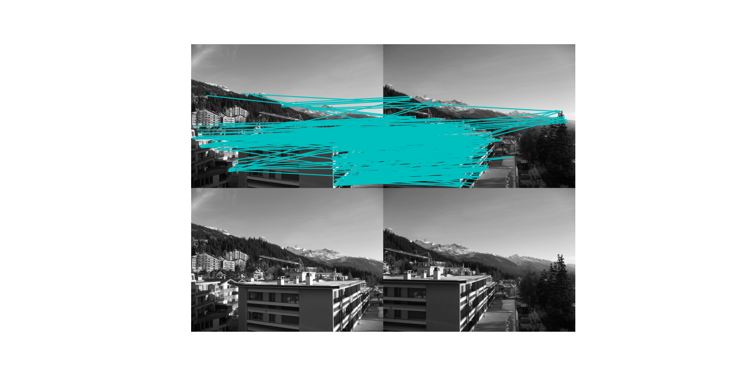
如图所示，该算法的结果存在一些不正确匹配。这是因为，与现代的一些方法相比，图像像素块的互相关矩阵具有较弱的描述性。实际运用中，我们通常使用更稳健的方法来处理这些对应匹配。这些描述符还有一个问题，它们不具有尺度不变性和旋转不变性，而算法中像素块的大小也会影响对应匹配的结果。

2.2 SIFT（ 尺度不变特征变换）

SIFT（ Scale-Invariant Feature Transform，尺度不变特征变换）是过去十年中最成功的图像局部描述子之一。

兴趣点

SIFT 特征使用高斯差分函数来定位兴趣点：
$$D(\mathbf{x},\sigma )=\left[G_{\kappa \sigma }(\mathbf{x})-G_{\sigma }(\mathbf{x})\right]\ast \mathbf{I}(\mathbf{x})=\left[G_{\kappa \sigma }-G_{\sigma }\right]\ast \mathbf{I}={\mathbf{I}}_{\kappa \sigma }-{\mathbf{I}}_{\sigma }$$

$G_{\sigma }$是上一章中介绍的二维高斯核，$I_{\sigma }$是使用$G_{\sigma }$模糊的灰度图像， κ 是决定相差尺度的常数。

兴趣点是在图像位置和尺度变化下 D(x,σ) 的最大值和最小值点。这些候选位置点通过滤波去除不稳定点。基于一些准则，比如认为低对比度和位于边上的点不是兴趣点，我们可以去除一些候选兴趣点。

描述子

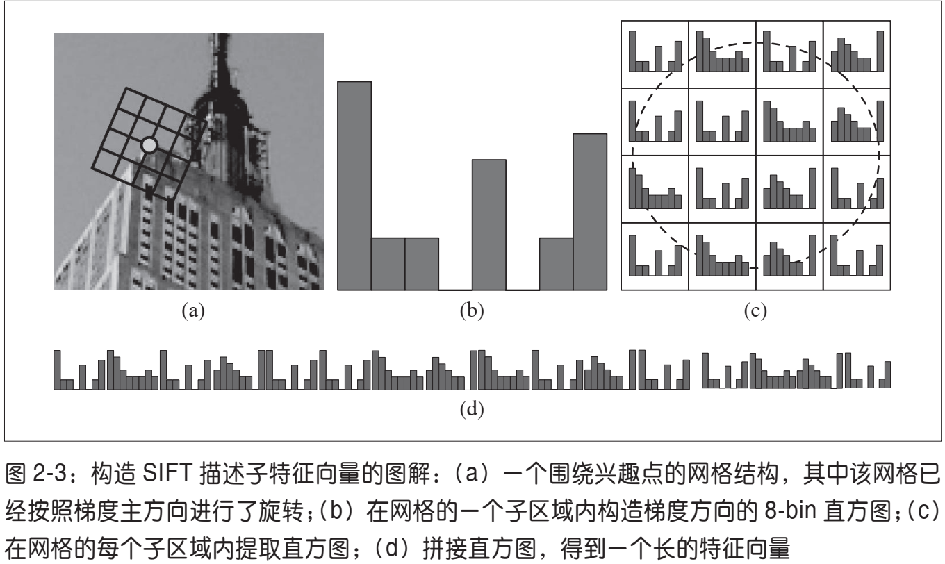
上面讨论的兴趣点（关键点）位置描述子给出了兴趣点的位置和尺度信息。为了实现旋转不变性，基于每个点周围图像梯度的方向和大小， SIFT 描述子又引入了参考方向。SIFT 描述子使用主方向描述参考方向。主方向使用方向直方图（以大小为权重）来度量。

为了对图像亮度具有稳健性，SIFT 描述子使用图像梯度（之前 Harris 描述子使用图像亮度信息计算归一化互相关矩阵）。 SIFT 描述子在每个像素点附近选取子区域网格，在每个子区域内计算图像梯度方向直方图。每个子区域的直方图拼接起来组成描述子向量。 SIFT 描述子的标准设置使用 4× 4 的子区域，每个子区域使用 8 个小区间的方向直方图，会产生共128 个小区间的直方图（ 4× 4× 8=128）。图 2-3 所示为描述子的构造过程。

检测兴趣点

先去下载开源工具包VLFeat这个网站

代码如下：

import os

def process_image(imagename,resultname,params="--edge-thresh 10 --peak-thresh 5"):
    """ 处理图像并将结果保存在文件里 """
 
    if imagename[-3:] != 'pgm':
        # create a pgm file
        im = Image.open(imagename).convert('L')
        im.save('tmp.pgm')
        imagename = 'tmp.pgm'
 
    cmmd = str("D:\python\exercise_data\ComputerVision\ch02\sift.exe " \
        +imagename+" --output="+resultname+" "+params)
    os.system(cmmd)
    print ('processed', imagename, 'to', resultname)

def read_features_from_file(filename):
    """ 读取特征属性值，然后将其以矩阵的形式返回 """
    
    f = loadtxt(filename)
    return f[:,:4],f[:,4:] # feature locations, descriptors

def plot_features(im,locs,circle=False):
    """ 显示带有特征的图像 """
 
    def draw_circle(c,r):
        t = arange(0,1.01,.01)*2*pi
        x = r*cos(t) + c[0]
        y = r*sin(t) + c[1]
        plot(x,y,'b',linewidth=2)
 
    imshow(im)
    if circle:
        for p in locs:
            draw_circle(p[:2],p[2]) 
    else:
        plot(locs[:,0],locs[:,1],'ob')
    axis('off')

def plot_harris_points(image,filtered_coords):
    """ Plots corners found in image. """
    
    gray()
    imshow(image)
    plot([p[1] for p in filtered_coords],
                [p[0] for p in filtered_coords],'*')
    axis('off')
    


from PCV.localdescriptors import harris

def siftMatching(fileName):
    """ 函数功能：sift特征变换
        参数说明: fileName__图片地址
        函数返回：无
    """
    img1 = array(Image.open(fileName[2]).convert('L'))
    gray()
    # SIFT特征
    process_image(fileName[2], 'empire.sift')
    l1, d1 = read_features_from_file('empire.sift')
    # 角点检测
    harrisimg = harris.compute_harris_response(img1)
    filtered_coords = harris.get_harris_points(harrisimg, 6)

    # 图片输出
    subplot(131)
    plot_features(img1, l1, circle=True), title('circle SIFT 特征',fontproperties=myfont)
    subplot(132)
    plot_features(img1, l1, circle=False), title('SIFT 特征',fontproperties=myfont)
    
    subplot(133)
    plot_harris_points(img1, filtered_coords),title(' Harris 角点',fontproperties=myfont)
    
    show()
    return

输出图片如下：

上面三幅图都是对一幅图像提取 SIFT 特征。分别是SIFT 特征、使用圆圈表示特征尺度的 SIFT 特征以及为了比较，对于同一幅图像提取 Harris 角点。
对比发现Harris描述点大多集中在窗户上而SIFT提取的特征则更全面一些。

匹配描述子

对于将一幅图像中的特征匹配到另一幅图像的特征，一种稳健的准则（同样是由Lowe 提出的）是使用这两个特征距离和两个最匹配特征距离的比率。相比于图像中的其他特征，该准则保证能够找到足够相似的唯一特征。使用该方法可以使错误的匹配数降低。

def matchDescribePoint(fileName):
    """ 函数功能：描述点匹配
        参数说明: fileName__图片地址
        函数返回：无
    """
    
    if len(sys.argv) >= 3:
        im1f, im2f = sys.argv[1], sys.argv[2]
    else:
        im1f = fileName[0]
        im2f = fileName[1]
    im1 = array(Image.open(im1f))
    im2 = array(Image.open(im2f))
    
    sift.process_image(im1f, 'out_sift_1.txt')
    l1, d1 = sift.read_features_from_file('out_sift_1.txt')
    figure()
    gray()
    subplot(121)
    sift.plot_features(im1, l1, circle=False)
    sift.process_image(im2f, 'out_sift_2.txt')
    l2, d2 = sift.read_features_from_file('out_sift_2.txt')
    subplot(122)
    sift.plot_features(im2, l2, circle=False)
    matches = sift.match_twosided(d1, d2)
    print('{} matches'.format(len(matches.nonzero()[0])))
    figure()
    gray()
    sift.plot_matches(im1, im2, l1, l2, matches, show_below=True)
    show()
      
    return

输出如下：

上面的图第一幅为两幅图片的特征点，下面的图片则表示的为连接图片中对应匹配的点以及他们的原图的展示。

2.3　匹配地理标记图像

2.3.1图像搜集

书里说了很多，但是我觉得其实就是在搜集图片，搜集数据。方法是从网上下载，为了下载处理好图片，我们要使用这些工具。我没有使用图中的方法，直接去网上下载了一些学校图片。应该也可以。

2.3.2 使用局部描述子匹配

def matchGeographyMark(path):
    """ 函数功能：匹配地理标记图像
        参数说明: path图片存储路径
        函数返回：无
    """  
    # path = "D:\\picture\\test_img3"

    imlist = get_imlist(path)

    nbr_images = len(imlist)
    featlist = [imname[:-4] + 'sift' for imname in imlist]
    for i, imname in enumerate(imlist):
        process_image(imname, featlist[i])
    
    matchscores = zeros((nbr_images, nbr_images))
    
    for i in range(nbr_images):
        for j in range(i, nbr_images):
            print('comparing ', imlist[i], imlist[j])
            l1, d1 = sift.read_features_from_file(featlist[i])
            l2, d2 = sift.read_features_from_file(featlist[j])
            matches = sift.match_twosided(d1, d2)
            nbr_matches = sum(matches > 0)
            print('number of matches = ', nbr_matches)
            matchscores[i, j] = nbr_matches
    print("The match scores is: \n", matchscores)
    
    for i in range(nbr_images):
        for j in range(i + 1, nbr_images):  # no need to copy diagonal
            matchscores[j, i] = matchscores[i, j]
    
    # poltGeographyMark(path, nbr_images,matchscores,imlist)
    return

在这里插入代码片输出结果如下：

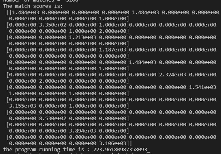
显示的是对应图片相似特征点的数量。后期根据这个特征点的数量对图片进行连接。

2.3.3 可视化连接图像

展示一下工具：

def plotDot():
    """ 函数功能：可视化链接打印测试
        参数说明: 无
        函数返回：无 
    """
    g = pydot.Dot(graph_type='graph')
    g.add_node(pydot.Node(str(0),fontcolor='transparent'))
    for i in range(5):
        # 添加节点
        g.add_node(pydot.Node(str(i+1)))
        #添加边
        g.add_edge(pydot.Edge(str(0),str(i+1)))
        for j in range(5):
            g.add_node(pydot.Node(str(j+1)+'-'+str(i+1)))
            g.add_edge(pydot.Edge(str(j+1)+'-'+str(i+1),str(j+1)))
    
    g.write_png('graph.jpg',prog='neato')
    
    return

输出结果如下：

实现我们图片的可视化连接：

from pylab import *
import pydot

def poltGeographyMark(path,datapath):
    """ 函数功能：打印地理标记连接关系
        参数说明: path__图片地址
                 dataPath__相似点数量矩阵存储地址
        函数返回：无
    """
    graphpath = r'C:/Users/haoqiao/Graphviz/bin'
    imlist = get_imlist(path)
    nbr_images = len(imlist)
    #loadtxt没办法加载float型
    # matchscores = loadtxt(datapath)
    
    # 以只读方式打开文件
    matchscores =[]
    with open(datapath, 'r') as f:
        
        numFeat = len(open(datapath).readline().split(','))
        for line in f.readlines():
            lineArr =[]
            curLine = line.strip().split(',')
            for index in range(numFeat):
                lineArr.append(float(curLine[index]))
            matchscores.append(lineArr)
    matchscores = array(matchscores)
    print(matchscores)

    # matchscores = mat(matchscores)
    # print(matchscores)
    # 可视化
    threshold = 1  # min number of matches needed to create link
    # 不使用默认的有向图
    g = pydot.Dot(graph_type='graph')  
    
    for i in range(nbr_images):
        for j in range(i + 1, nbr_images):
            if matchscores[i, j] > threshold:
                # first image in pair
                im = Image.open(imlist[i])
                im.thumbnail((100, 100))
                filename = graphpath +str(i) + '.png'
                im.save(filename)  # need temporary files of the right size
                g.add_node(pydot.Node(str(i), fontcolor='transparent', shape='rectangle', image= filename))
                # second image in pair
                im = Image.open(imlist[j])
                im.thumbnail((100, 100))
                filename = graphpath + str(j) + '.png'
                im.save(filename)  # need temporary files of the right size
                g.add_node(pydot.Node(str(j), fontcolor='transparent', shape='rectangle', image= filename))
                g.add_edge(pydot.Edge(str(i), str(j)))
        g.write_png(r'test1.png')
    
    return

def get_imlist(path):
    imlist = []
    for f in os.listdir(path):
        if f.endswith('.jpg'):
            imlist.append(os.path.join(path,f))

    return imlist


def matchGeographyMark(path):
    """ 函数功能：匹配地理标记图像
        参数说明: path图片存储路径
        函数返回：无
    """  

    imlist = get_imlist(path)

    nbr_images = len(imlist)
    featlist = [imname[:-4] + 'sift' for imname in imlist]
    for i, imname in enumerate(imlist):
        process_image(imname, featlist[i])
    
    matchscores = zeros((nbr_images, nbr_images))
    
    for i in range(nbr_images):
        for j in range(i, nbr_images):
            print('comparing ', imlist[i], imlist[j])
            l1, d1 = read_features_from_file(featlist[i])
            l2, d2 = read_features_from_file(featlist[j])
            matches = match_twosided(d1, d2)
            nbr_matches = sum(matches > 0)
            print('number of matches = ', nbr_matches)
            matchscores[i, j] = nbr_matches
    print("The match scores is: \n", matchscores)
    
    for i in range(nbr_images):
        for j in range(i + 1, nbr_images):  # no need to copy diagonal
            matchscores[j, i] = matchscores[i, j]
    # 转为整形
    # matchscores = matchscores.astype(int)
    savetxt(r'matchscoers.txt',matchscores,delimiter=',')

    # poltGeographyMark(path, nbr_images,matchscores,imlist)
    return

def plotDot():
    """ 函数功能：可视化链接打印测试
        参数说明: 无
        函数返回：无 
    """
    g = pydot.Dot(graph_type='graph')
    g.add_node(pydot.Node(str(0),fontcolor='transparent'))
    for i in range(5):
        # 添加节点
        g.add_node(pydot.Node(str(i+1)))
        #添加边
        g.add_edge(pydot.Edge(str(0),str(i+1)))
        for j in range(5):
            g.add_node(pydot.Node(str(j+1)+'-'+str(i+1)))
            g.add_edge(pydot.Edge(str(j+1)+'-'+str(i+1),str(j+1)))
    
    g.write_png('graph.jpg',prog='neato')
    
    return

def main():
    fileName = [r'C:/hqq/document/python/ComputerVision/ch02/figure/crans_1_small.jpg',
                r'C:/hqq/document/python/ComputerVision/ch02/figure/crans_2_small.jpg',
                r'C:/hqq/document/python/ComputerVision/ch02/figure/empire.jpg',
                r'C:/hqq/document/python/ComputerVision/ch02/figure/school1.jpg',
                r'C:/hqq/document/python/ComputerVision/ch02/figure/school2.jpg'
                
                ]

    path=r"C:/hqq/document/python/computervision/ch02/schoolpicture"
    dataPath = r"C:/hqq/document/python/computervision/ch02/matchscoers.txt"

    # cornerDetection(fileName)
    # searchCorrespondingPoint(fileName)
    # siftMatching(fileName)

    # matchDescribePoint(fileName)
    # plotDot()
    matchGeographyMark(path)
    poltGeographyMark(path,dataPath)

    return
    

代码能跑，且能输出，但是输出结果不对。后面再进行调试一下。我认为问题可能是出现在了（##）好像也不对，输出不对打印当然不对。后面再看一下。

输出结果如下：

输出的特征匹配后的图片和我们认为的有很大的差异。换一些图片试一下。

忠告：图片不要用太大的，不然很崩溃。。。。

输出如下：

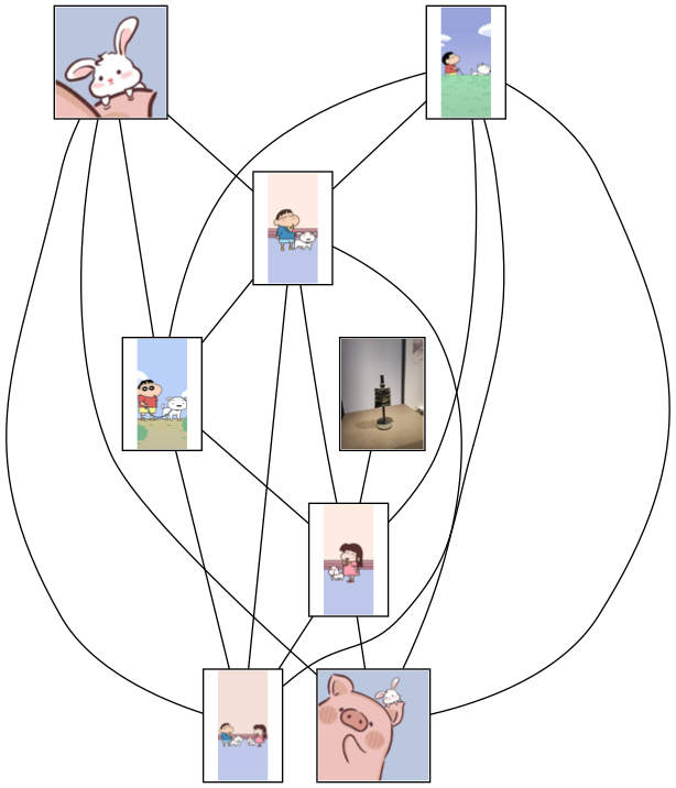
有两张图片被丢掉了？？
将阈值改为

threshold = 0

仍然有一幅图片没有链接起来。

修改一下判断调节为

if matchscores[i, j] >= threshold:

修改判断条件后全部显示出来了。他只将有关联的图像输出，完全没有关联的就不会输出。

代码调试过程遇到的问题我记录在了Python学习笔记（六）中，有问题可以看一下。

2.4小结

本章主要内容也是最重要的就是引入了图片角点相关概念，后面随之介绍了角点检测算法、Harris矩阵、基于Harris提出的角点检测器。后面利用该检测器找出图像间的对应角点。当然仅检测出图像兴趣点就依此匹配图像间的角点是不可能的，所以我们引出来另外一个概念，就是描述子信息，并且给出一个比较这些描述子的方法。后面我们发现这个描述子还能改进，所以提出了SIFT（ Scale-Invariant Feature Transform，尺度不变特征变换）后面就是利用该方法对两幅图像进行SIFT的特征匹配。

代码及图片如下：

链接：https://pan.baidu.com/s/1QS6gervAbO61cOTH3ckpBQ?pwd=muxv
提取码：muxv

需要自取