R统计绘图-变量分组相关性网络图(igraph)
一、数据准备
数据是21个土壤样本的环境因子,细菌和真菌丰度数据。
library(tidyverse)
library(igraph)
library(psych)
### 1.1 观测-变量数据表
data<- read.csv("data.csv",header = TRUE,
row.names = 1,
check.names=FALSE,
comment.char = "")
head(data)
### 1.2 变量分类表
type = read.csv("type.csv",header = TRUE,check.names = FALSE)
type # 变量分类信息

图1|观测-变量数据表。行为观测样本,列为变量。
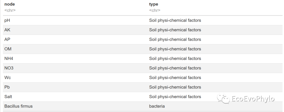
图2|变量分类表。node为变量名,type为变量分类。
二、确定相关性关系
2.1 计算相关性系数
psych包的corr.test()计算相关性系数、显著性检验和p值校正。
### 2.1 计算相关性系数,建议使用spearman系数。
cor <- corr.test(data, use = "pairwise",method="spearman",adjust="holm", alpha=.05,ci=FALSE) # ci=FALSE,不进行置信区间计算,数据量较大时,可以加快计算速度。
cor.r <- data.frame(cor$r) # 提取R值
cor.p <- data.frame(cor$p) # 提取p值
colnames(cor.r) = rownames(cor.r)
colnames(cor.p) = rownames(cor.p) # 变量名称中存在特殊字符,为了防止矩阵行名与列名不一致,必须运行此代码。
write.csv(cor.r,"cor.r.csv",quote = FALSE,col.names = NA,row.names = TRUE) # 保存结果到本地
write.csv(cor.p,"cor.p.csv",quote = FALSE,col.names = NA,row.names = TRUE)
knitr::kable(
  head(cor.r),
  caption = "cor.r"
)
head(cor.p)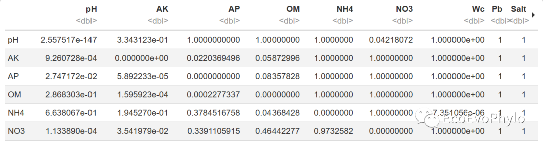
图3|相关性p值矩阵。
2.2 确定相关性关系
### 2.2 确定相关性关系 保留p<=0.05且abs(r)>=0.6的变量间相关关系
#cor.r[abs(cor.r) < 0.6 | cor.p > 0.05] = 0
#cor.r = as.matrix(cor.r)
#g = graph_from_adjacency_matrix(cor.r,mode = "undirected",weighted = TRUE,diag = FALSE)
#### 将数据转换为long format进行过滤,后面绘制网络图需要节点和链接数据,在这一步可以完成格式整理
cor.r$node1 = rownames(cor.r)
cor.p$node1 = rownames(cor.p)
r = cor.r %>%
  gather(key = "node2", value = "r", -node1) %>%
  data.frame()
p = cor.p %>%
  gather(key = "node2", value = "p", -node1) %>%
  data.frame()
head(r)
head(p)
#### 将r和p值合并为一个数据表
cor.data <- merge(r,p,by=c("node1","node2"))
cor.data
#### 保留p<=0.05且abs(r)>=0.6的变量间相关关系,并添加网络属性
cor.data <- cor.data %>%
  filter(abs(r) >= 0.6, p <= 0.05, node1 != node2) %>%
  mutate(
    linetype = ifelse(r > 0,"positive","negative"), # 设置链接线属性,可用于设置线型和颜色。
    linesize = abs(r) # 设置链接线宽度。
    ) # 此输出仍有重复链接,后面需进一步去除。
head(cor.data)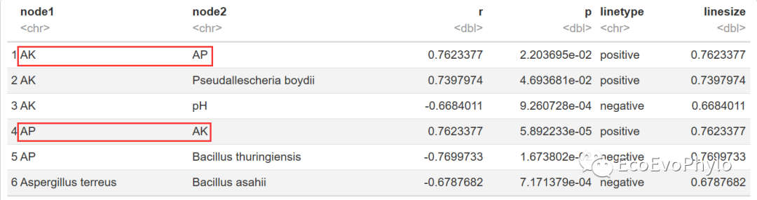
图4|未删除重复链接前的链接属性表,cor.data。
三、构建网络图结构数据
3.1 网络图节点属性整理
此步构建网络之后,还需要将网络图转换为简单图,去除重复链接。
### 3.1 网络图节点属性整理
#### 计算每个节点具有的链接数
c(as.character(cor.data$node1),as.character(cor.data$node2)) %>%
  as_tibble() %>%
  group_by(value) %>%
  summarize(n=n()) -> vertices
colnames(vertices) <- c("node", "n")
head(vertices)
#### 添加变量分类属性
vertices %>%
  select(-n) %>% # 因为此处的n不准确,所以先删除。
  left_join(type,by="node") -> vertices
#### 网络图中节点会按照节点属性文件的顺序依次绘制,为了使同类型变量位置靠近,按照节点属性对节点进行排序。
vertices$type = factor(vertices$type,levels = unique(vertices$type))
vertices = arrange(vertices,type)
write.csv(vertices,"vertices.csv",quote = FALSE,col.names = NA,row.names = FALSE)
head(vertices)
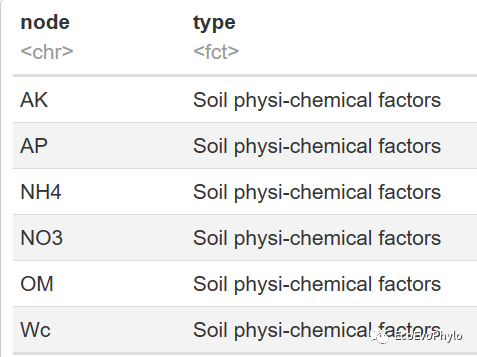
图5|节点属性表,vertices。
3.2 构建graph结构数据
### 3.2 构建graph结构数据
g <- graph_from_data_frame(cor.data, vertices = vertices, directed = FALSE )
g
vcount(g) # 节点数目:82
ecount(g) # 链接数:297
#get.vertex.attribute(g) # 查看graph中包含的节点属性
#get.edge.attribute(g) # 查看graph中包含的链接属性
图6|未删除重复链接前的graph,g。
3.3 简单图
### 3.3 简单图
is.simple(g) # 非简单图,链接数会偏高,所以需要转换为简单图。
E(g)$weight <- 1
g <- igraph::simplify(g,
                      remove.multiple = TRUE,
                      remove.loops = TRUE,
                      edge.attr.comb = "first")
#g <- delete.vertices(g,which(degree(g) == 0)) # 删除孤立点
is.simple(g)
E(g)$weight <- 1
is.weighted(g)
vcount(g) # 节点数目:21
ecount(g) # 链接数:33
3.4 计算节点链接数
### 3.4 计算节点链接数
V(g)$degree <- degree(g)
#vertex.attributes(g)
#edge.attributes(g)
g
图7|删除重复链接后的graph,g。
3.5 保存graph数据到本地
### 3.5 graph保存到本地
write.graph(g,file = "all.gml",format="gml") # 直接保存graph结构,gml能保存的graph信息最多。
net.data  <- igraph::as_data_frame(g, what = "both")$edges # 提取链接属性
write.csv(net.data,"net.data.csv",quote = FALSE,col.names = NA,row.names = FALSE) # 保存结果到本地。
head(net.data)
vertices  <- igraph::as_data_frame(g, what = "both")$vertices # 提取节点属性
write.csv(vertices,"vertices.csv",quote = FALSE,col.names = NA,row.names = FALSE)
head(vertices) # 直接读入之前保存的链接和节点属性文件,之后可直接生成graph或用于其他绘图软件绘图。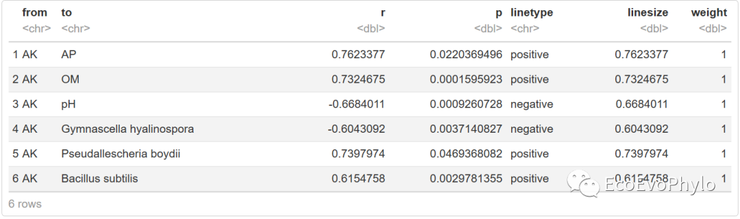
图8|无重复链接属性表,net.data。
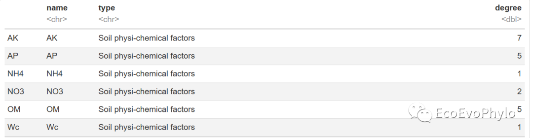
图9|添加degree的新节点属性表,vertices。
四、绘制分组网络图
图属性:1) 节点根据分类属性填充颜色和背景色;2) 节点大小按degree设置;3) 链接线根据正负相关性设置颜色;4) 链接线宽度根据abs(r)设置。
绘图前先确定网络图中的节点位置,即计算每个节点的(x,y)坐标,igraph包中有多个图布局计算函数,可根据不同的算法计算出网络图中的节点坐标位置。可以多尝试几种布局方式,找到最适合自己数据的布局。
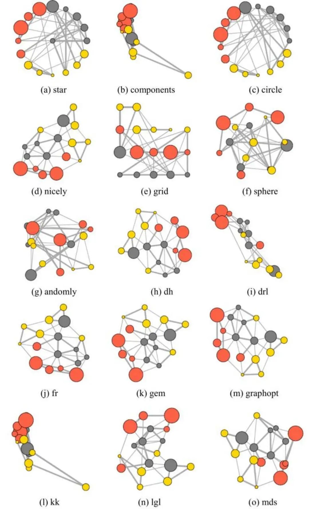
图10|网络图布局方式。来自《R语言数据可视化之美》。
4.1 设置网络图布局
### 4.1 准备网络图布局数据
#?layout_in_circle # 帮助信息中,有其它布局函数。
layout1 <- layout_in_circle(g) # 径向布局适合节点较少的数据。
layout2 <- layout_with_fr(g) # fr布局。
layout3 <- layout_on_grid(g) # grid布局。
head(layout1)
4.2 设置绘图颜色
### 4.2 设置绘图颜色
#?rgb() # 可以将RGB值转换为16进制颜色名称。
#### 设置节点与分组背景色
color <- c(rgb(65,179,194,maxColorValue = 255),
          rgb(255,255,0,maxColorValue = 255),
          rgb(201,216,197,maxColorValue = 255))
names(color) <- unique(V(g)$type) # 将颜色以节点分类属性命名
V(g)$point.col <- color[match(V(g)$type,names(color))] # 设置节点颜色。
#names(color2) <- unique(V(g)$type) # 如果想要节点颜色与背景颜色不一致,则可以为节点单独设置一个颜色集。
#V(g)$point.col <- color2[match(V(g)$type,names(color2))]
#### 边颜色按照相关性正负设置
#E(g)$color <- ifelse(E(g)$linetype == "positive",rgb(255,215,0,maxColorValue = 255),"gray50")
E(g)$color <- ifelse(E(g)$linetype == "positive","red",rgb(0,147,0,maxColorValue = 255))

图11|graph绘图布局,layout1。
4.3 径向布局网络图
与其他布局相比,径向网络图比较适合节点较少的数据。
### 4.3 绘制径向布局网络图
pdf("network_group_circle.pdf",family = "Times",width = 10,height = 12)
par(mar=c(5,2,1,2))
plot.igraph(g, layout=layout1,#更多参数设置信息?plot.igraph查看。
##节点颜色设置参数##
     vertex.color=V(g)$point.col,
     vertex.frame.color ="black",
     vertex.border=V(g)$point.col,
##节点大小设置参数##
     vertex.size=V(g)$n,
##节点标签设置参数##
     vertex.label=g$name,
     vertex.label.cex=0.8,
     vertex.label.dist=0, # 标签距离节点中心的距离,0表示标签在节点中心。
#vertex.label.degree = pi/4, # 标签对于节点的位置,0-右,pi-左,-pi/2-上,pi/2-下。
     vertex.label.col="black",
##设置节点分组列表,绘制分组背景色##
     mark.groups =list(V(g)$name[V(g)$type %in% names(color)[1]],
                       V(g)$name[V(g)$type %in% names(color)[2]],
                       V(g)$name[V(g)$type %in% names(color)[3]]
                       ), #
     mark.col=color,
     mark.border=color,
#mark.expand = 1, # 设置背景阴影大小,1表示阴影边框刚全包节点。
##链接属性参数以edge*开头##
     edge.arrow.size=0.5,
     edge.width=abs(E(g)$r)*2,
     edge.curved = TRUE
     )
##设置图例,与plot.igraph()函数一起运行##
legend(
  title = "Type",
  list(x = min(layout1[,1])-0.2,
y = min(layout1[,2])-0.17), # 图例的位置需要根据自己的数据进行调整,后面需要使用AI手动调整。
  legend = c(unique(V(g)$type)),
  fill = color,
#pch=1
)
legend(
  title = "|r-value|",
  list(x = min(layout1[,1])+0.4,
y = min(layout1[,2])-0.17),
  legend = c(0.6,0.8,1.0),
  col = "black",
  lty=1,
  lwd=c(0.6,0.8,1.0)*2,
)
legend(
  title = "Correlation (±)",
  list(x = min(layout1[,1])+0.8,
y = min(layout1[,2])-0.17),
  legend = c("positive","negative"),
  col = c("red",rgb(0,147,0,maxColorValue = 255)),
  lty=1,
  lwd=1
)
legend(
  title = "Degree",
  list(x = min(layout1[,1])+1.2,
y = min(layout1[,2])-0.17),
  legend = c(1,seq(0,8,2)[-1]),# V(g)$degree。
  col = "black",
  pch=1,
  pt.lwd=1,
  pt.cex=c(1,seq(0,8,2)[-1])
)
dev.off()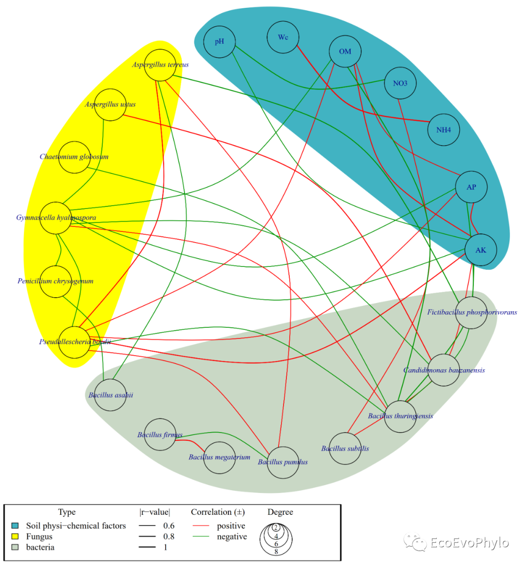
图12|径向布局分组网络图,network_group_circle.pdf。图例位置需要AI或pdf编辑器调整一下。不想标签放在节点上,也可AI调整。
4.4 绘制fr布局网络图
fr布局(Fruchterman-Reingold 算法的力导向布局)适合变量较多的数据。
### 4.4 绘制fr布局网络图-不添加背景色
pdf("network_group_fr.pdf",family = "Times",width = 10,height = 12)
par(mar=c(5,2,1,2))
plot.igraph(g, layout=layout2,#更多参数设置信息?plot.igraph查看。
##节点颜色设置参数##
     vertex.color=V(g)$point.col,
     vertex.frame.color ="black",
     vertex.border=V(g)$point.col,
##节点大小设置参数##
     vertex.size=V(g)$n,
##节点标签设置参数##
     vertex.label=g$name,
     vertex.label.cex=0.8,
#vertex.label.dist=0, # 标签距离节点中心的距离,0表示标签在节点中心。
#vertex.label.degree = 0, # 标签对于节点的位置,0-右,pi-左,-pi/2-上,pi/2-下。
     vertex.label.col="black",
##链接属性参数以edge*开头##
     edge.arrow.size=0.5,
     edge.width=abs(E(g)$r)*2,
     edge.curved = TRUE
     )
##设置图例,与plot.igraph()函数一起运行##
legend(
  title = "Type",
  list(x = min(layout1[,1])-0.2,
y = min(layout1[,2])-0.17), # 图例的位置需要根据自己的数据进行调整,后面需要使用AI手动调整。
  legend = c(unique(V(g)$type)),
  fill = color,
#pch=1
)
legend(
  title = "|r-value|",
  list(x = min(layout1[,1])+0.4,
y = min(layout1[,2])-0.17),
  legend = c(0.6,0.8,1.0),
  col = "black",
  lty=1,
  lwd=c(0.6,0.8,1.0)*2,
)
legend(
  title = "Correlation (±)",
  list(x = min(layout1[,1])+0.8,
y = min(layout1[,2])-0.17),
  legend = c("positive","negative"),
  col = c("red",rgb(0,147,0,maxColorValue = 255)),
  lty=1,
  lwd=1
)
legend(
  title = "Degree",
  list(x = min(layout1[,1])+1.2,
y = min(layout1[,2])-0.17),
  legend = c(1,seq(0,8,2)[-1]),# max(V(g)$degree)
  col = "black",
  pch=1,
  pt.lwd=1,
  pt.cex=c(1,seq(0,8,2)[-1])
)
dev.off()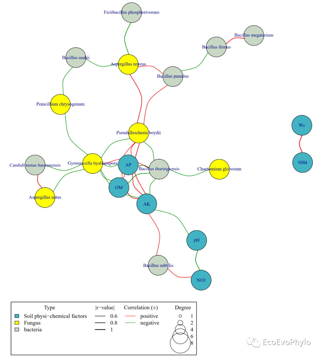
图13|fr布局变量分组网络图,network_group_fr.pdf。
4.5 绘制grid布局网络图
### 4.5 绘制grid布局网络图-不添加背景色
pdf("network_group_grid.pdf",family = "Times",width = 10,height = 12)
par(mar=c(5,2,1,2))
plot.igraph(g, layout=layout3,#更多参数设置信息?plot.igraph查看。

##节点颜色设置参数##
     vertex.color=V(g)$point.col,
     vertex.frame.color ="black",
     vertex.border=V(g)$point.col,
##节点大小设置参数##
     vertex.size=V(g)$n,
##节点标签设置参数##
     vertex.label=g$name,
     vertex.label.cex=0.8,
     vertex.label.dist=0, # 标签距离节点中心的距离,0表示标签在节点中心。
     vertex.label.degree = pi/2, # 标签对于节点的位置,0-右,pi-左,-pi/2-上,pi/2-下。
     vertex.label.col="black",
##链接属性参数以edge*开头##
     edge.arrow.size=0.5,
     edge.width=abs(E(g)$r)*2,
     edge.curved = TRUE,
#edge.label.x = # 链接线标签位置横坐标。
#edge.label.y = # 链接线标签位置纵坐标。
     )
##设置图例,与plot.igraph()函数一起运行##
legend(
  title = "Type",
  list(x = min(layout1[,1])-0.2,
y = min(layout1[,2])-0.17), # 图例的位置需要根据自己的数据进行调整,后面需要使用AI手动调整。
  legend = c(unique(V(g)$type)),
  fill = color,
#pch=1
)
legend(
  title = "|r-value|",
  list(x = min(layout1[,1])+0.4,
y = min(layout1[,2])-0.17),
  legend = c(0.6,0.8,1.0),
  col = "black",
  lty=1,
  lwd=c(0.6,0.8,1.0)*2,
)
legend(
  title = "Correlation (±)",
  list(x = min(layout1[,1])+0.8,
y = min(layout1[,2])-0.17),
  legend = c("positive","negative"),
  col = c("red",rgb(0,147,0,maxColorValue = 255)),
  lty=1,
  lwd=1
)
legend(
  title = "Degree",
  list(x = min(layout1[,1])+1.2,
y = min(layout1[,2])-0.17),
  legend = c(1,seq(0,8,2)[-1]),# max(V(g)$degree)
  col = "black",
  pch=1,
  pt.lwd=1,
  pt.cex=c(1,seq(0,8,2)[-1])
)
dev.off()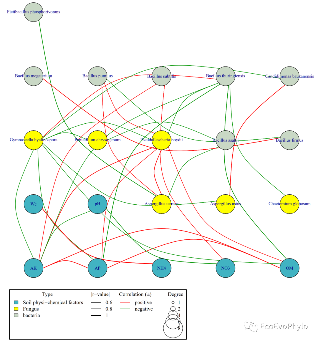
图14|grid布局变量分组网络图,network_group_grid.pdf。
参考资料
https://hiplot-academic.com/basic/network-igraph
微信公众号后台回复"network_group"或QQ群文件获取数据和代码。
原文链接:R统计绘图-变量分组相关性网络图(igraph)

EcoEvoPhylo :主要分享微生物生态和phylogenomics的数据分析教程。扫描上方二维码,关注EcoEvoPhylo。让我们大家一起学习,互相交流,共同进步。
知乎 | 生态媛
学术交流QQ群 | 438942456
学术交流微信群 | jingmorensheng412
加好友时,请备注姓名-单位-研究方向。
推荐阅读
R绘图-物种、环境因子相关性网络图(简单图、提取子图、修改图布局参数、物种-环境因子分别成环径向网络图)
R统计绘图-分子生态相关性网络分析(拓扑属性计算,ggraph绘图)
R中进行单因素方差分析并绘图
R统计绘图-多变量单因素非参数差异检验及添加显著性标记图
R统计绘图-单因素Kruskal-Wallis检验
R统计绘图-单、双、三因素重复测量方差分析[Translation]
R统计-多变量单因素参数、非参数检验及多重比较
R统计-多变量双因素参数、非参数检验及多重比较
R绘图-KEGG功能注释组间差异分面条形图
R绘图-相关性分析及绘图
R绘图-相关性系数图
R统计绘图-环境因子相关性热图
R绘图-RDA排序分析
R统计-VPA分析(RDA/CCA)
R统计绘图-RDA分析、Mantel检验及绘图
R统计-PCA/PCoA/db-RDA/NMDS/CA/CCA/DCA等排序分析教程
R统计-正态性分布检验[Translation]
R统计-数据正态分布转换[Translation]
R统计-方差齐性检验[Translation]
R统计-Mauchly球形检验[Translation]
R统计绘图-混合方差分析[Translation]
R统计绘图-协方差分析[Translation]
R统计绘图-RDA分析、Mantel检验及绘图
R统计绘图-factoextra包绘制及美化PCA结果图
R统计绘图-环境因子相关性+mantel检验组合图(linkET包介绍1)
R统计绘图-随机森林分类分析及物种丰度差异检验组合图
机器学习-分类随机森林分析(randomForest模型构建、参数调优、特征变量筛选、模型评估和基础理论等)