1. t-sne可视化基本概念

1. 流形学习的设计目的
   Manifold learning is an approach to non-linear dimensionality reduction. Algorithms for this task are based on the idea that the dimensionality of many data sets is only artificially high.
   Manifold是一种非线性降维的方法。这个任务的算法是基于这样一种想法，即许多数据集的维数只是人为地偏高。
   Manifold Learning can be thought of as an attempt to generalize linear frameworks like PCA to be sensitive to non-linear structure in data. Though supervised variants exist, the typical manifold learning problem is unsupervised: it learns the high-dimensional structure of the data from the data itself, without the use of predetermined classifications.
   Manifold可以被认为是一种推广线性框架的尝试，如PCA，以敏感的非线性数据结构。虽然有监督变量存在，但典型的Manifold问题是非监督的:它从数据本身学习数据的高维结构，而不使用预定的分类。
2. 数据降维与可视化
   t-distributed Stochastic Neighbor Embedding(t-SNE)，即t-分布随机邻居嵌入。t-SNE是一个可视化高维数据的工具。它将数据点之间的相似性转化为联合概率，并试图最小化低维嵌入和高维数据联合概率之间的Kullback-Leibler差异。t-SNE有一个非凸的代价函数，即通过不同的初始化，我们可以得到不同的结果。强烈建议使用另一种降维方法(如密集数据的PCA或稀疏数据的集群svd)来减少维数到一个合理的数量(如50)，如果特征的数量非常高。这将抑制一些噪声，加快样本间成对距离的计算。
3. 主要特点以及功能作用–判别数据是否可分
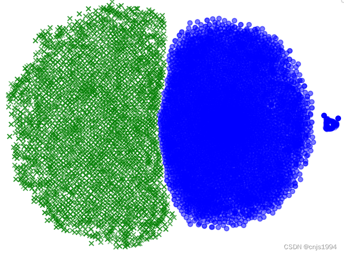
   t-SNE是目前来说效果最好的数据降维与可视化方法，但是它的缺点也很明显，比如：占内存大，运行时间长。但是，当我们想要对高维数据进行分类，又不清楚这个数据集有没有很好的可分性（即同类之间间隔小，异类之间间隔大），可以通过t-SNE投影到2维或者3维的空间中观察一下。如果在低维空间中具有可分性，则数据是可分的；如果在高维空间中不具有可分性，可能是数据不可分，也可能仅仅是因为不能投影到低维空间。t-SNE（TSNE）的原理是将数据点之间的相似度转换为概率。原始空间中的相似度由高斯联合概率表示，嵌入空间的相似度由“学生t分布”表示。

2. sklearn.manifold.TSNE函数的参数说明

参数

• n_componentsint, default=2: 嵌入空间的尺寸。
• min_grad_normfloat, default=1e-7:如果梯度范数低于这个阈值，优化将停止。
• init{‘random’, ‘pca’} or ndarray of shape (n_samples, n_components), default=’random’:初始化的嵌入。可能的选项是’ random ‘，’ pca '和numpy数组的形状(n_samples, n_components)。PCA初始化不能与预先计算的距离一起使用，而且通常比随机初始化更全局稳定。

3. 基于tensorflow2卷积网络t-SNE特征可视化

import numpy as np
import pandas as pd

from sklearn.model_selection import cross_val_score, train_test_split, KFold
import matplotlib.pyplot as plt
from sklearn.metrics import confusion_matrix
from sklearn.preprocessing import LabelEncoder
import itertools
import tensorflow
from tensorflow.keras.optimizers import SGD
from tensorflow.keras.layers import Dense, Activation, Flatten, Convolution1D, Dropout, MaxPooling1D, BatchNormalization
from tensorflow.keras.models import model_from_json
from tensorflow.keras.utils import plot_model
from tensorflow.python.keras.utils import np_utils
from tensorflow.keras.models import Sequential
from sklearn.manifold import TSNE

"""
一维卷积神经网络 输入为信号片段；输出为轴承的故障类别；
做的t-sne可视化demo程序
点靠颜色和形状区分 x o
"""

# 载入数据
df = pd.read_csv(r'C:\Users\86139\PycharmProjects\pythonProject_at_tsinghua\TF2_t_SNE\14改.csv')
#####################################################################
# 定义神经网络
def baseline_model():
    model = Sequential()
    model.add(Convolution1D(16, 128, strides=1, input_shape=(1024, 1), padding="same"))
    model.add(Activation('tanh'))
    model.add(MaxPooling1D(2, strides=2, padding='same'))

    # model.add(BatchNormalization(axis=-1, momentum=0.99, epsilon=0.001, center=True, scale=True, beta_initializer='zeros', gamma_initializer='ones', moving_mean_initializer='zeros', moving_variance_initializer='ones', beta_regularizer=None, gamma_regularizer=None, beta_constraint=None, gamma_constraint=None))
    model.add(Convolution1D(32, 3, padding='same'))
    model.add(
        BatchNormalization(axis=-1, momentum=0.99, epsilon=0.001, center=True, scale=True, beta_initializer='zeros',
                           gamma_initializer='ones', moving_mean_initializer='zeros',
                           moving_variance_initializer='ones', beta_regularizer=None, gamma_regularizer=None,
                           beta_constraint=None, gamma_constraint=None))
    model.add(Activation('tanh'))
    model.add(MaxPooling1D(2, strides=2, padding='same'))

    model.add(Flatten())
    model.add(Dropout(0.3))
    model.add(Dense(60, activation='tanh'))
    model.add(Dense(2, activation='softmax'))
    print(model.summary())
    sgd = SGD(lr=0.01, nesterov=True, decay=1e-6, momentum=0.9)
    model.compile(loss='categorical_crossentropy', optimizer='adam', metrics=['accuracy'])
    return model

# 模型训练
nb_epoch = 10
model = baseline_model()
estimator = model.fit(X_train, Y_train, epochs=nb_epoch, validation_data=(X_test, Y_test), batch_size=32)
num_layer=1
layer = tensorflow.keras.backend.function([model.layers[0].input], [model.layers[num_layer].output])

f1 = layer([X_train])[0]
np.set_printoptions(threshold=np.inf)
print(f"f1-shape: {f1.shape}")
# print(f1)
f2 = f1.reshape(f1.shape[0]*f1.shape[2], f1.shape[1])
# print(f2)
num = f1.shape[-1]
print(num)

def get_data(f1):
    # digits = datasets.load_digits(n_class=10)
    digits = 2
    data = f2  # digits.data		# 图片特征
    label = K  # digits.target		# 图片标签
    n_samples = f1.shape[0] * f1.shape[2]
    n_features = f1.shape[1]  # data.shape		# 数据集的形状
    return data, label, n_samples, n_features

data, label, n_samples, n_features = get_data(f1)  # 调用函数，获取数据集信息
print('Starting compute t-SNE Embedding...')
ts = TSNE(n_components=2, init='pca', random_state=0)

# t-SNE降维
result = ts.fit_transform(data)

# 数据归一化与可视化
x_min, x_max = np.min(result, 0), np.max(result, 0)
data = (result - x_min) / (x_max - x_min)  # 对数据进行归一化处理
#####################################################################
# 把标签读出来--因为就是增倍，且序号顺序未变
label2 = np.repeat(label, 16)
map_marker = {0.0: 'o', 1.0: 'x'}
markers = list(map(lambda x: map_marker[x], label2))
map_color = {0.0: 'b', 1.0: 'g'}
colors = list(map(lambda x: map_color[x], label2))

mscatter(data[:, 0], data[:, 1], s=20, c=colors, cmap='tab10', m=markers, alpha=0.3)
plt.legend()
plt.show()

可视化部分参考了下这篇博客[2]

参考

[1] https://blog.csdn.net/m0_47410750/article/details/123119544?spm=1001.2014.3001.5502
[2] https://blog.csdn.net/u014571489/article/details/102667570