分位数回归的求解

分位数回归实际上是一种特殊的${\ell }_1$回归问题，特别地，当所求分位数$\tau =0.5$时就是中位数回归。

将分位数回归看做是线性规划问题来求解

一般的，线性回归问题可以写为${\ell }_p$范数线性回归，简称为${\ell }_p$回归:
$$\underset{x\in {\mathbb{R}}^n}{\mathrm{argmin}}||\mathbf{A}\mathbf{x}-\mathbf{b}|{|}_p$$
其中$\mathbf{A}\in {\mathbb{R}}^{m\times n},b\in {\mathbb{R}}^m$，$||v|{|}_p=({\sum }_i|{\mathbf{v}}_i{|}^p{)}^{1/p}$表示${\ell }_p$范数
那么从中位数回归的角度来看，损失函数就是绝对损失($p=1$):
$$\underset{x\in {\mathbb{R}}^n}{\mathrm{argmin}}||\mathbf{A}\mathbf{x}-\mathbf{b}||$$
考虑一个两参数的分位数回归优化问题
$$\begin{array}{c}\hat{\beta }=\underset{(b_0,b_1)\in {\mathbb{R}}^2}{\mathrm{argmin}}\left\{\sum _{i=1}^n|y_i-b_0-b_1{x}_i|\right\}\end{array}$$
$\tau$分位数时更一般的形式
$$\hat{\beta }(\tau )=\underset{\mathbf{b}\in {\mathbb{R}}^{m\times n}}{\mathrm{argmin}}\sum _{i=1}^n{\rho }_{\tau }(y_i-{\mathbf{x}}_i^{\top }\mathbf{b})$$
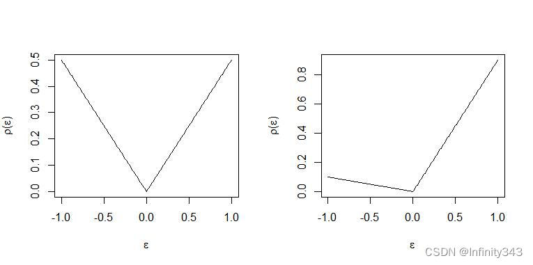
其中$\tau \in (0,1)$是分位数. ${\rho }_{\tau }(\cdot )$是check function(又称检查函数):
$${\rho }_{\tau }(u)=u(\tau -I(u<0))$$
定义${\epsilon }_i=y_i-{\mathbf{x}}_i^{\top }\mathbf{b}$为第$i$个残差，则优化目标$(1)$可以转化为残差的形式
$$\begin{array}{c}\hat{\beta }=\underset{(b_0,b_1)\in {\mathbb{R}}^2}{\mathrm{argmin}}\left\{\sum _{i=1}^n{\epsilon }_i\right\}\end{array}$$
将上式改写：
$$\begin{array}{c}\sum _{i=1}^n{\rho }_{\tau }(\epsilon {}_i)=\sum _{i=1}^n\tau {\epsilon }_i^{+}+(1-\tau )|{\epsilon }_i^{-}|\end{array}$$
由于分位数回归使用的是绝对损失函数，残差恒正，所以将其拆分为正部${\epsilon }_i^{+}=u_i={\epsilon }_{i}I(y_i-{\mathbf{x}}_i^{\top }\mathbf{b}>0),{\epsilon }_i^{-}=v_i={\epsilon }_{i}I(y_i-{\mathbf{x}}_i^{\top }\mathbf{b}<0)$
可见，回归残差的正部被赋予了$\tau$权重，负部被赋予$(1-\tau )$的权重，令$\tau =0.5$就是等权，所以中位数回归又是分位数回归的一个特例。

不难看出，${\ell }_1$回归问题在零点处不可导，所以OLS方法不可用，但可以将其划为线性回归问题进行求解。对于一个线性规划问题其标准形式为
$$\begin{gathered} \underset{z}{\min }{c}^{\top }z \\ \mathrm{subject}\mathrm{to}\mathbf{A}z={\mathbf{b}}^{\ast },z\ge 0 \end{gathered}$$
这里的$b^{\ast }$带上星号是为了区分开回归参数$b$. 从定义来看，线性回归标准型要求所有决策变量大于零，显然残差是有正有负的，为满足上述条件，回忆之前对残差正负部的定义：
$${\epsilon }_i=u_i-v_i$$
其中正部$u_i=\max (0,{\epsilon }_i)$负部$v_i=\max (0,-{\epsilon }_i)=|{\epsilon }_i|I_{\epsilon <0}$。
此时式(3)改写为
$$\sum _{i=1}^n{\rho }_{\tau }({\epsilon }_i)=\sum _{i-1}^n{u}_i\tau +v_i(1-\tau )=\tau 1_n^{\top }\mathbf{u}+(1-\tau )1_n^{\top }\mathbf{v}$$
其中$\mathbf{u}=(u_1,\dots ,u_n{)}^{\top },\mathbf{v}=(v_1,\dots ,v_n{)}^{\top }$, $1_n$是$n\times 1$的全一向量。为记号方便，之后的向量或矩阵将不再加粗，而是通过取消下标来表示。若样本量为$N$参数个数为$K$，令$u,v$为松弛变量，则会有$N$个等式约束
$$y_i-x_i^{\top }b={\epsilon }_i=u_i-v_{i}i=1,\dots N$$
上式就可以改写为一个线性规划：
$$\underset{b\in {\mathbb{R}}^K,u\in {\mathbb{R}}_{+}^N,v\in {\mathbb{R}}_{+}^N}{\min }\left\{\tau 1_N^{\top }u+(1-\tau )1_N^{\top }v\mid y_i=x_{i}b+u_i-v_i,i=1,\dots ,N\right\}$$
注意到，上式中参数$b\in {\mathbb{R}}^K$不能保证非负，所以也需要将$b$分解为正负部
$$b=b^{+}-b^{-}$$
其中$b^{+}=\max (0,b),b^{-}=\max (0,-b)$, 该$N$个等式约束以矩阵表达(更直观)：
$$y:=\left[\begin{array}{c}{y}_1\\ ⋮\\ y_N\end{array}\right]=\left[\begin{array}{c}{\mathbf{x}}_1^{\top }\\ ⋮\\ {\mathbf{x}}_N^{\top }\end{array}\right]\left(b^{+}-b^{-}\right)+{\mathbf{I}}_{N}u-{\mathbf{I}}_{N}v$$
其中${\mathbf{I}}_N=diag(1_N)$.将$\mathbf{x}$写为矩阵继续简化表达
$$\mathbf{X}\left(b^{+}-b^{-}\right)+{\mathbf{I}}_{N}u-{\mathbf{I}}_{N}v=\left[\mathbf{X},-\mathbf{X},{\mathbf{I}}_N,-{\mathbf{I}}_N\right]\left[\begin{array}{c}{b}^{+}\\ b^{-}\\ u\\ v\end{array}\right]$$
可以看到现在我们有$N$个等式约束，$2K$个参数(因为参数被分为了正负部，所以乘2)，另外还有$2N$个松弛变量：
$$A:=[\mathbf{X}-\mathbf{X}{\mathbf{I}}_N-{\mathbf{I}}_N]$$
符合标准型的约束条件为：
$$b^{\ast }=A\left[\begin{array}{c}{b}^{+}\\ b^{-}\\ u\\ v\end{array}\right]=Az$$
因为$b^{+}$和$b^{-}$仅通过约束影响最小化问题(优化目标中并不存在$b$)，所以必须引入维度为$2K\times 1$的 $0$ 作为系数向量 $c$ 的一部分，可以适当地定义为
$$c=\left[\begin{array}{c}0\\ \tau 1_N\\ (1-\tau )1_N\end{array}\right]$$
这样目标函数就是
$$c^{\top }z=\underset{=0}{\underbrace{0^{\top }\left(b^{+}-b^{-}\right)}}+\tau 1_N^{\top }u+(1-\tau )1_N^{\top }v=\sum _{i=1}^N{\rho }_{\tau }\left({\epsilon }_i\right).$$
显然此时已经识别出了线性规划标准型的所有因素，利用R或python就可以实现求解

getwd()
setwd('C:/Users/beida/Desktop')
base=read.table("rent98_00.txt",header=TRUE)
attach(base)
library(quantreg)
library(lpSolve)
tau <- 0.5


# only one covariate
X <- cbind(1, base$area)  #设计阵X
K <- ncol(X)   #列数量，即参数个数
N <- nrow(X)   #行数量，即样本量(等式约束量)

A <- cbind(X, -X, diag(N), -diag(N)) #优化系数
c <- c(rep(0, 2*ncol(X)), tau*rep(1, N), (1-tau)*rep(1, N))  #目标函数系数
b <- base$rent_euro  #响应变量Y
const_type <- rep("=", N) #N个等式约束

linprog <- lp("min", c, A, const_type, b)
beta <- linprog$sol[1:K] - linprog$sol[(1:K+K)] #
beta


rq(rent_euro ~ area, tau=tau, data=base)

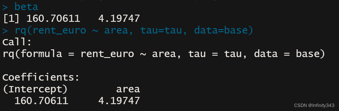
可以看到线性规划求解的结果与quantreg包的rq函数得到了相同的解。
python同理

import io

import numpy as np
import pandas as pd
import requests
np.


url = "http://freakonometrics.free.fr/rent98_00.txt"
s = requests.get(url).content
base = pd.read_csv(io.StringIO(s.decode('utf-8')), sep='\t')


tau = 0.5

from cvxopt import matrix, solvers

X = pd.DataFrame(columns=[0, 1])
X[1] = base["area"]  # data points for independent variable area
#X[2] = base["year"]  # data points for independent variable year
X[0] = 1  # intercept

K = X.shape[1]
N = X.shape[0]

# equality constraints - left hand side

A1 = X.to_numpy()  # intercepts & data points - positive weights
A2 = X.to_numpy() * -1  # intercept & data points - negative weights
A3 = np.identity(N)  # error - positive
A4 = np.identity(N) * -1  # error - negative

A = np.concatenate((A1, A2, A3, A4), axis=1)  # all the equality constraints

# equality constraints - right hand side
b = base["rent_euro"].to_numpy()

# goal function - intercept & data points have 0 weights
# positive error has tau weight, negative error has 1-tau weight
c = np.concatenate((np.repeat(0, 2 * K), tau * np.repeat(1, N), (1 - tau) * np.repeat(1, N)))

# converting from numpy types to cvxopt matrix

Am = matrix(A)
bm = matrix(b)
cm = matrix(c)

# all variables must be greater than zero
# adding inequality constraints - left hand side
n = Am.size[1]
G = matrix(0.0, (n, n))
G[:: n + 1] = -1.0

# adding inequality constraints - right hand side (all zeros)
h = matrix(0.0, (n, 1))

# solving the model
sol = solvers.lp(cm, G, h, Am, bm, solver='glpk')

x = sol['x']

# both negative and positive components get values above zero, this gets fixed here
beta = x[0:K] - x[K : 2 * K]

print(beta)

• 思考
  从R的运行情况来看，线性规划的求解速度显著慢于rq函数，这与求解方法有关。rq提供了以下方法来求解分位数回归：

the algorithmic method used to compute the fit. There are several options:

• “br” The default method is the modified version of the Barrodale and Roberts algorithm for
  $l_1$-regression, used by l1fit in S, and is described in detail in Koenker and d’Orey(1987, 1994), default = “br”. This is quite efficient for problems up to several thousand observations, and may be used to compute the full quantile regression process. It also implements a scheme for computing confidence intervals for the estimated parameters, based on inversion of a rank test described in Koenker(1994).

• “fn” For larger problems it is advantageous to use the Frisch–Newton interior point method “fn”. This is described in detail in Portnoy and Koenker(1997).

• “pfn” For even larger problems one can use the Frisch–Newton approach after preprocessing “pfn”. Also described in detail in Portnoy and Koenker(1997), this method is primarily well-suited for large n, small p problems, that is when the parametric dimension of the model is modest.

• “sfn” For large problems with large parametric dimension it is often advantageous to use method “sfn” which also uses the Frisch-Newton algorithm, but exploits sparse algebra to compute iterates. This is especially helpful when the model includes factor variables that, when expanded, generate design matrices that are very sparse. At present options for inference, i.e. summary methods are somewhat limited when using the “sfn” method. Only the option se = “nid” is currently available, but I hope to implement some bootstrap options in the near future.

• “fnc” Another option enables the user to specify linear inequality constraints on the fitted coefficients; in this case one needs to specify the matrix R and the vector r representing the constraints in the form Rb \geq rRb≥r. See the examples below.

• “conquer” For very large problems especially those with large parametric dimension, this option provides a link to the conquer of He, Pan, Tan, and Zhou (2020). Calls to summary when the fitted object is computed with this option invoke the multiplier bootstrap percentile method of the conquer package and can be considerably quicker than other options when the problem size is large. Further options for this fitting method are described in the conquer package. Note that this option employs a smoothing form of the usual QR objective function so solutions may be expected to differ somewhat from those produced with the other options.

• “pfnb” This option is intended for applications with large sample sizes and/or moderately fine tau grids. It uses a form of preprocessing to accelerate the solution process. The loop over taus occurs inside the Fortran call and there should be more efficient than other methods in large problems.

• “qfnb” This option is like the preceeding one except that it doesn’t use the preprocessing option.

• “ppro” This option is an R prototype of the pfnb and is offered for historical/interpretative purposes, but probably should be considered deprecated.

• “lasso” There are two penalized methods: “lasso” and “scad” that implement the lasso penalty and Fan and Li smoothly clipped absolute deviation penalty, respectively. These methods should probably be regarded as experimental. Note: weights are ignored when the method is penalized.

可见求解方法之多，运行速度也不尽相同。但需要注意的是对于当前问题，单纯形法是很难甚至是无法求解的

simplex(c, A3 = A, b3 = b, maxi = TRUE,  n.iter =200, eps = 1e-4)

> No feasible solution could be found

我们只选取了两个回归系数，样本量为4571，单纯形法的计算时间就超过了5分钟，且没有得到可行解(尽管降低了解的精度要求)。
后续将继续更新别的求解算法。