扩散模型实战（九）：使用CLIP模型引导和控制扩散模型

推荐阅读列表：

 扩散模型实战（一）：基本原理介绍

扩散模型实战（二）：扩散模型的发展

扩散模型实战（三）：扩散模型的应用

扩散模型实战（四）：从零构建扩散模型

扩散模型实战（五）：采样过程

扩散模型实战（六）：Diffusers DDPM初探

扩散模型实战（七）：Diffusers蝴蝶图像生成实战

扩散模型实战（八）：微调扩散模型

上篇文章中介绍了如何微调扩散模型，有时候微调的效果仍然不能满足需求，比如图片编辑，3D模型输出等都需要对生成的内容进行控制，本文将初步探索一下如何控制扩散模型的输出。

我们将使用在LSUM bedrooms数据集上训练并在WikiArt数据集上微调的模型，首先加载模型来查看一下模型的生成效果：

!pip install -qq diffusers datasets accelerate wandb open-clip-torch

import numpy as npimport torchimport torch.nn.functional as Fimport torchvisionfrom datasets import load_datasetfrom diffusers import DDIMScheduler, DDPMPipelinefrom matplotlib import pyplot as pltfrom PIL import Imagefrom torchvision import transformsfrom tqdm.auto import tqdm

device = (    "mps"    if torch.backends.mps.is_available()    else "cuda"    if torch.cuda.is_available()    else "cpu")

# 载入一个预训练过的管线pipeline_name = "johnowhitaker/sd-class-wikiart-from-bedrooms"image_pipe = DDPMPipeline.from_pretrained(pipeline_name).to(device)　# 使用DDIM调度器，仅用40步生成一些图片scheduler = DDIMScheduler.from_pretrained(pipeline_name)scheduler.set_timesteps(num_inference_steps=40)　# 将随机噪声作为出发点x = torch.randn(8, 3, 256, 256).to(device)　# 使用一个最简单的采样循环for i, t in tqdm(enumerate(scheduler.timesteps)):    model_input = scheduler.scale_model_input(x, t)    with torch.no_grad():        noise_pred = image_pipe.unet(model_input, t)["sample"]    x = scheduler.step(noise_pred, t, x).prev_sample　# 查看生成结果，如图5-10所示grid = torchvision.utils.make_grid(x, nrow=4)plt.imshow(grid.permute(1, 2, 0).cpu().clip(-1, 1) * 0.5 + 0.5)

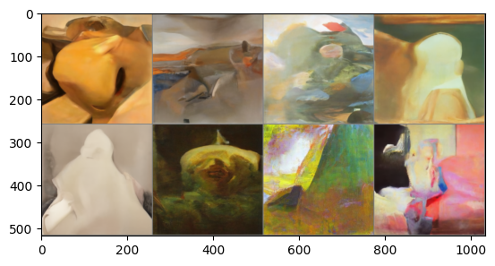
       正如上图所示，模型可以生成一些图片，那么如何进行控制输出呢？下面我们以控制图片生成绿色风格为例介绍AIGC模型控制：

       思路是：定义一个均方误差损失函数，让生成的图片像素值尽量接近目标颜色；

def color_loss(images, target_color=(0.1, 0.9, 0.5)):    """给定一个RGB值，返回一个损失值，用于衡量图片的像素值与目标颜色相差多少； 这里的目标颜色是一种浅蓝绿色，对应的RGB值为(0.1, 0.9, 0.5)"""    target = (        torch.tensor(target_color).to(images.device) * 2 - 1    )  # 首先对target_color进行归一化，使它的取值区间为(-1, 1)     target = target[        None, :, None, None    ]  # 将所生成目标张量的形状改为(b, c, h, w)，以适配输入图像images的 # 张量形状    error = torch.abs(        images - target    ).mean()  # 计算图片的像素值以及目标颜色的均方误差    return error

接下来，需要修改采样循环操作，具体操作步骤如下：

1. 创建输入图像X，并设置requires_grad设置为True；

2. 计算“去噪”后的图像X0；

3. 将“去噪”后的图像X0传递给损失函数；

4. 计算损失函数对输入图像X的梯度；

5. 在使用调度器之前，先用计算出来的梯度修改输入图像X，使输入图像X朝着减少损失值的方向改进

实现上述步骤有两种方法：

方法一：从UNet中获取噪声预测，并将输入图像X的requires_grad属性设置为True，这样可以充分利用内存（因为不需要通过扩散模型追踪梯度），但是这会导致梯度的精度降低；

方法二：先将输入图像X的requires_grad属性设置为True，然后传递给UNet并计算“去噪”后的图像X0；

下面分别看一下这两种方法的效果：

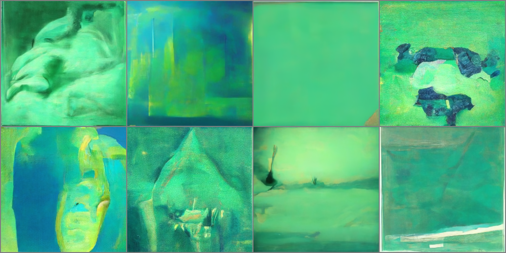
# 第一种方法　# guidance_loss_scale用于决定引导的强度有多大guidance_loss_scale = 40  # 可设定为5~100的任意数字　x = torch.randn(8, 3, 256, 256).to(device)　for i, t in tqdm(enumerate(scheduler.timesteps)):　    # 准备模型输入    model_input = scheduler.scale_model_input(x, t)　    # 预测噪声    with torch.no_grad():        noise_pred = image_pipe.unet(model_input, t)["sample"]　    # 设置x.requires_grad为True    x = x.detach().requires_grad_()　    # 得到“去噪”后的图像    x0 = scheduler.step(noise_pred, t, x).pred_original_sample　    # 计算损失值    loss = color_loss(x0) * guidance_loss_scale    if i % 10 == 0:        print(i, "loss:", loss.item())　    # 获取梯度    cond_grad = -torch.autograd.grad(loss, x)[0]　    # 使用梯度更新x    x = x.detach() + cond_grad　    # 使用调度器更新x    x = scheduler.step(noise_pred, t, x).prev_sample# 查看结果grid = torchvision.utils.make_grid(x, nrow=4)im = grid.permute(1, 2, 0).cpu().clip(-1, 1) * 0.5 + 0.5Image.fromarray(np.array(im * 255).astype(np.uint8))

# 输出0 loss: 29.3701839447021510 loss: 12.11665058135986320 loss: 11.64170455932617230 loss: 11.78276252746582

# 第二种方法：在模型预测前设置好x.requires_gradguidance_loss_scale = 40x = torch.randn(4, 3, 256, 256).to(device)　for i, t in tqdm(enumerate(scheduler.timesteps)):　    # 首先设置好requires_grad    x = x.detach().requires_grad_()    model_input = scheduler.scale_model_input(x, t)　    # 预测    noise_pred = image_pipe.unet(model_input, t)["sample"]　    # 得到“去噪”后的图像    x0 = scheduler.step(noise_pred, t, x).pred_original_sample　    # 计算损失值    loss = color_loss(x0) * guidance_loss_scale    if i % 10 == 0:        print(i, "loss:", loss.item())　    # 获取梯度    cond_grad = -torch.autograd.grad(loss, x)[0]　    # 根据梯度修改x    x = x.detach() + cond_grad　    # 使用调度器更新x    x = scheduler.step(noise_pred, t, x).prev_sample　　grid = torchvision.utils.make_grid(x, nrow=4)im = grid.permute(1, 2, 0).cpu().clip(-1, 1) * 0.5 + 0.5Image.fromarray(np.array(im * 255).astype(np.uint8))

# 输出0 loss: 27.6226882934570310 loss: 16.84250640869140620 loss: 15.5464210510253930 loss: 15.545379638671875

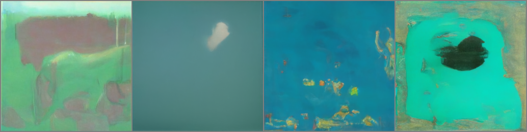
       从上图看出，第二种方法效果略差，但是第二种方法的输出更接近训练模型所使用的数据，也可以通过修改guidance_loss_scale参数来增强颜色的迁移效果。

CLIP控制图像生成

       虽然上述方式可以引导和控制图像生成某种颜色，但现在LLM更主流的方式是通过Prompt（仅仅打几行字描述需求）来得到自己想要的图像，那么CLIP是一个不错的选择。CLIP是有OpenAI开发的图文匹配大模型，由于这个过程是可微分的，所以可以将其作为损失函数来引导扩散模型。

使用CLIP控制图像生成的基本流程如下：

1. 使用CLIP模型对Prompt表示为512embedding向量；

2. 在扩散模型的生成过程中需要多次执行如下步骤：

   1）生成多个“去噪”图像；

   2）对生成的每个“去噪”图像用CLIP模型进行embedding，并对Prompt embedding和图像的embedding进行对比；

   3）计算Prompt和“去噪”后图像的梯度，使用这个梯度先更新输入图像X，然后再使用调度器更新X；

   加载CLIP模型

import open_clip　clip_model, _, preprocess = open_clip.create_model_and_transforms(    "ViT-B-32", pretrained="openai")clip_model.to(device)　# 图像变换：用于修改图像尺寸和增广数据，同时归一化数据，以使数据能够适配CLIP模型 tfms = torchvision.transforms.Compose(    [        torchvision.transforms.RandomResizedCrop(224),# 随机裁剪        torchvision.transforms.RandomAffine(5),       # 随机扭曲图片        torchvision.transforms.RandomHorizontalFlip(),# 随机左右镜像， # 你也可以使用其他增广方法        torchvision.transforms.Normalize(            mean=(0.48145466, 0.4578275, 0.40821073),            std=(0.26862954, 0.26130258, 0.27577711),        ),    ])　# 定义一个损失函数，用于获取图片的特征，然后与提示文字的特征进行对比def clip_loss(image, text_features):    image_features = clip_model.encode_image(        tfms(image)    )  # 注意施加上面定义好的变换    input_normed = torch.nn.functional.normalize(image_features.       unsqueeze(1), dim=2)    embed_normed = torch.nn.functional.normalize(text_features.       unsqueeze(0), dim=2)    dists = (        input_normed.sub(embed_normed).norm(dim=2).div(2).           arcsin().pow(2).mul(2)    )  # 使用Squared Great Circle Distance计算距离    return dists.mean()

      下面是引导模型生成图像的过程，步骤与上述类似，只需要把color_loss()替换成CLIP的损失函数

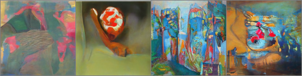
prompt = "Red Rose (still life), red flower painting"　# 读者可以探索一下这些超参数的影响guidance_scale = 8n_cuts = 4　# 这里使用稍微多一些的步数scheduler.set_timesteps(50)　# 使用CLIP从提示文字中提取特征text = open_clip.tokenize([prompt]).to(device)with torch.no_grad(), torch.cuda.amp.autocast():    text_features = clip_model.encode_text(text)　x = torch.randn(4, 3, 256, 256).to(    device) 　for i, t in tqdm(enumerate(scheduler.timesteps)):　    model_input = scheduler.scale_model_input(x, t)　    # 预测噪声    with torch.no_grad():        noise_pred = image_pipe.unet(model_input, t)["sample"]　    cond_grad = 0　    for cut in range(n_cuts):　        # 设置输入图像的requires_grad属性为True        x = x.detach().requires_grad_()　        # 获得“去噪”后的图像        x0 = scheduler.step(noise_pred, t, x).pred_original_sample　        # 计算损失值        loss = clip_loss(x0, text_features) * guidance_scale　        # 获取梯度并使用n_cuts进行平均        cond_grad -= torch.autograd.grad(loss, x)[0] / n_cuts　    if i % 25 == 0:        print("Step:", i, ", Guidance loss:", loss.item())　    # 根据这个梯度更新x    alpha_bar = scheduler.alphas_cumprod[i]    x = (        x.detach() + cond_grad * alpha_bar.sqrt()    )  # 注意这里的缩放因子　    # 使用调度器更新x    x = scheduler.step(noise_pred, t, x).prev_sample　　grid = torchvision.utils.make_grid(x.detach(), nrow=4)im = grid.permute(1, 2, 0).cpu().clip(-1, 1) * 0.5 + 0.5Image.fromarray(np.array(im * 255).astype(np.uint8))

# 输出Step: 0 , Guidance loss: 7.418107986450195Step: 25 , Guidance loss: 7.085518836975098

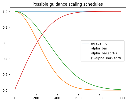
       上述生成的图像虽然不够完美，但可以调整一些超参数，比如梯度缩放因子alpha_bar.sqrt()，虽然理论上存在所谓的正确的缩放这些梯度方法，但在实践中仍需要实验来检验，下面介绍一些常用的方案：

plt.plot([1 for a in scheduler.alphas_cumprod], label="no scaling")plt.plot([a for a in scheduler.alphas_cumprod], label="alpha_bar")plt.plot([a.sqrt() for a in scheduler.alphas_cumprod],     label="alpha_bar.sqrt()")plt.plot(    [(1 - a).sqrt() for a in scheduler.alphas_cumprod], label="(1-     alpha_bar).sqrt()")plt.legend()