Pytorch从零开始实战10
Pytorch从零开始实战——ResNet-50算法实战
本系列来源于365天深度学习训练营
原作者K同学
文章目录
- Pytorch从零开始实战——ResNet-50算法实战
- 环境准备
- 数据集
- 模型选择
- 开始训练
- 可视化
- 模型预测
- 总结
环境准备
本文基于Jupyter notebook,使用Python3.8,Pytorch2.0.1+cu118,torchvision0.15.2,需读者自行配置好环境且有一些深度学习理论基础。本次实验的目的是理解ResNet-50模型。
第一步,导入常用包
import torch
import torch.nn as nn
import matplotlib.pyplot as plt
import torchvision
import torchvision.transforms as transforms
import torchvision.datasets as datasets
import torch.nn.functional as F
import random
from time import time
import numpy as np
import pandas as pd
import datetime
import gc
import os
import copy
import warnings
os.environ['KMP_DUPLICATE_LIB_OK']='True'  # 用于避免jupyter环境突然关闭
torch.backends.cudnn.benchmark=True  # 用于加速GPU运算的代码
设置随机数种子
torch.manual_seed(428)
torch.cuda.manual_seed(428)
torch.cuda.manual_seed_all(428)
random.seed(428)
np.random.seed(428)
检查设备对象
device = torch.device("cuda" if torch.cuda.is_available() else "cpu")
device, torch.cuda.device_count() # # (device(type='cuda'), 2)
数据集
本次数据集是使用鸟的图片,分别有四种类别的鸟,根据鸟的类别名称存放在不同的文件夹中。
使用pathlib查看类别
import pathlib
data_dir = './data/bird_photos/'
data_dir = pathlib.Path(data_dir) # 转成pathlib.Path对象
data_paths = list(data_dir.glob('*'))
classNames = [str(path).split("/")[2] for path in data_paths]
classNames # ['Black Throated Bushtiti', 'Cockatoo', 'Black Skimmer', 'Bananaquit']
使用transforms对数据集进行统一处理,并且根据文件夹名映射对应标签
all_transforms = transforms.Compose([transforms.Resize([224, 224]),transforms.ToTensor(),transforms.Normalize(mean=[0.485, 0.456, 0.406], std=[0.229, 0.224, 0.225]) # 标准化
])total_data = datasets.ImageFolder("./data/bird_photos/", transform=all_transforms)
total_data.class_to_idx# {'Bananaquit': 0,# 'Black Skimmer': 1,# 'Black Throated Bushtiti': 2,# 'Cockatoo': 3}
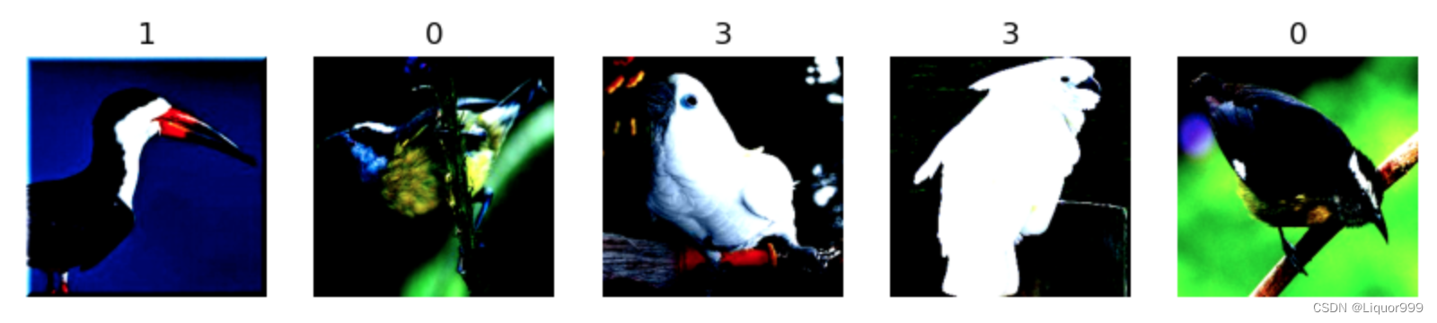
随机查看5张图片
def plotsample(data):fig, axs = plt.subplots(1, 5, figsize=(10, 10)) #建立子图for i in range(5):num = random.randint(0, len(data) - 1) #首先选取随机数,随机选取五次#抽取数据中对应的图像对象,make_grid函数可将任意格式的图像的通道数升为3,而不改变图像原始的数据#而展示图像用的imshow函数最常见的输入格式也是3通道npimg = torchvision.utils.make_grid(data[num][0]).numpy()nplabel = data[num][1] #提取标签 #将图像由(3, weight, height)转化为(weight, height, 3),并放入imshow函数中读取axs[i].imshow(np.transpose(npimg, (1, 2, 0))) axs[i].set_title(nplabel) #给每个子图加上标签axs[i].axis("off") #消除每个子图的坐标轴plotsample(total_data)
根据8比2划分数据集和测试集,并且利用DataLoader划分批次和随机打乱
train_size = int(0.8 * len(total_data))
test_size  = len(total_data) - train_size
train_ds, test_ds = torch.utils.data.random_split(total_data, [train_size, test_size])batch_size = 32
train_dl = torch.utils.data.DataLoader(train_ds,batch_size=batch_size,shuffle=True,)
test_dl = torch.utils.data.DataLoader(test_ds,batch_size=batch_size,shuffle=True,)len(train_dl.dataset), len(test_dl.dataset) # (452, 113)
模型选择
ResNet(Residual Network)是一种深度神经网络架构,由微软亚洲研究院的研究员Kaiming He等人于2015年提出。ResNet的设计主要解决了深度神经网络训练过程中的梯度消失和梯度爆炸等问题,使得训练更深的网络变得更为可行。
ResNet的关键创新点是引入了残差学习(Residual Learning)的概念。在传统的网络中,每一层的输入都是由前一层输出直接得到的,而ResNet则通过引入残差块(Residual Block)改变了这种方式。
残差块包含了一个跳跃连接(skip connection),将输入直接添加到网络的输出,形成了残差学习的结构。当输入为x,经过一个残差块后的输出为H(x),则残差块的计算方式可以表示为:H(x)=F(x)+x,其中,F(x)表示残差块的映射函数。由于存在跳跃连接,即直接将输入x加到输出上,这种结构使得神经网络能够学习恒等映射,即H(x)=x,从而更容易学习到恒等映射的变化部分,有助于减轻梯度爆炸或梯度消失问题。
ResNet的整体结构由多个残差块组成,包括一些卷积层、批归一化(Batch Normalization)和非线性激活函数。在深度网络中,ResNet的设计使得可以训练非常深的模型。
本次实验的ResNet-50有两个基本的块,分别名为Conv Block和Identity Block,借用K同学所绘制的图片。
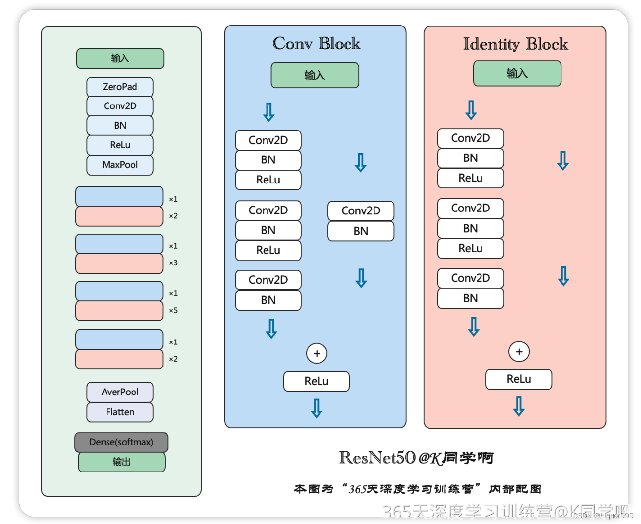
首先构建ResNet中的恒等块,恒等块是ResNet中的基本构建模块,用于在网络中引入残差学习,这个模块将输入x保存一份为t,x进行三个卷积,最终进行跳跃连接,将x和t相加。
class IdentityBlock(nn.Module):def __init__(self, in_channels, out_channels, kernel_size):super(IdentityBlock, self).__init__()self.conv1 = nn.Conv2d(in_channels, out_channels[0], kernel_size=1)self.bn1 = nn.BatchNorm2d(out_channels[0])self.relu1 = nn.ReLU()self.conv2 = nn.Conv2d(out_channels[0], out_channels[1], kernel_size=kernel_size, padding=1)self.bn2 = nn.BatchNorm2d(out_channels[1])self.relu2 = nn.ReLU()self.conv3 = nn.Conv2d(out_channels[1], out_channels[2], kernel_size=1)self.bn3 = nn.BatchNorm2d(out_channels[2])self.relu4 = nn.ReLU()def forward(self, x):t = xx = self.conv1(x)x = self.bn1(x)x = self.relu1(x)x = self.conv2(x)x = self.bn2(x)x = self.relu2(x)x = self.conv3(x)x = self.bn3(x)x += tx = self.relu4(x)return x
下面构建ResNet中的卷积模块,与恒等模块类似,不过t也经过一次卷积。
class ConvBlock(nn.Module):def __init__(self, in_channels, out_channels, kernel_size, strides=(2, 2)):super(ConvBlock, self).__init__()self.conv1 = nn.Conv2d(in_channels, out_channels[0], kernel_size=1, stride=strides)self.bn1 = nn.BatchNorm2d(out_channels[0])self.relu1 = nn.ReLU()self.conv2 = nn.Conv2d(out_channels[0], out_channels[1], kernel_size=kernel_size, padding=1)self.bn2 = nn.BatchNorm2d(out_channels[1])self.relu2 = nn.ReLU()self.conv3 = nn.Conv2d(out_channels[1], out_channels[2], kernel_size=1)self.bn3 = nn.BatchNorm2d(out_channels[2])self.conv = nn.Conv2d(in_channels, out_channels[2], kernel_size=1, stride=strides)self.bn = nn.BatchNorm2d(out_channels[2])self.relu4 = nn.ReLU()def forward(self, x):t = xx = self.conv1(x)x = self.bn1(x)x = self.relu1(x)x = self.conv2(x)x = self.bn2(x)x = self.relu2(x)x = self.conv3(x)x = self.bn3(x)t = self.conv(t)t = self.bn(t)x += tx = self.relu4(x)return x
构建ResNet50,使用上面的恒等块和卷积块,能够构建很深的网络模型。
class ResNet50(nn.Module):def __init__(self, input_shape=(3, 224, 224), num_classes=1000):super(ResNet50, self).__init__()self.conv1 = nn.Conv2d(input_shape[0], 64, kernel_size=7, stride=2, padding=3)self.bn_conv1 = nn.BatchNorm2d(64)self.relu = nn.ReLU()self.maxpool = nn.MaxPool2d(kernel_size=3, stride=2, padding=1)self.conv2 = ConvBlock(64, [64, 64, 256], kernel_size=3, strides=(1, 1))self.identity_block1 = IdentityBlock(256, [64, 64, 256], kernel_size=3)self.identity_block2 = IdentityBlock(256, [64, 64, 256], kernel_size=3)self.conv3 = ConvBlock(256, [128, 128, 512], kernel_size=3)self.identity_block3 = IdentityBlock(512, [128, 128, 512], kernel_size=3)self.identity_block4 = IdentityBlock(512, [128, 128, 512], kernel_size=3)self.identity_block5 = IdentityBlock(512, [128, 128, 512], kernel_size=3)self.conv4 = ConvBlock(512, [256, 256, 1024], kernel_size=3)self.identity_block6 = IdentityBlock(1024, [256, 256, 1024], kernel_size=3)self.identity_block7 = IdentityBlock(1024, [256, 256, 1024], kernel_size=3)self.identity_block8 = IdentityBlock(1024, [256, 256, 1024], kernel_size=3)self.identity_block9 = IdentityBlock(1024, [256, 256, 1024], kernel_size=3)self.identity_block10 = IdentityBlock(1024, [256, 256, 1024], kernel_size=3)self.conv5 = ConvBlock(1024, [512, 512, 2048], kernel_size=3)self.identity_block11 = IdentityBlock(2048, [512, 512, 2048], kernel_size=3)self.identity_block12 = IdentityBlock(2048, [512, 512, 2048], kernel_size=3)self.avg_pool = nn.AvgPool2d(kernel_size=7)self.fc = nn.Linear(2048, num_classes)def forward(self, x):x = self.conv1(x)x = self.bn_conv1(x)x = self.relu(x)x = self.maxpool(x)x = self.conv2(x)x = self.identity_block1(x)x = self.identity_block2(x)x = self.conv3(x)x = self.identity_block3(x)x = self.identity_block4(x)x = self.identity_block5(x)x = self.conv4(x)x = self.identity_block6(x)x = self.identity_block7(x)x = self.identity_block8(x)x = self.identity_block9(x)x = self.identity_block10(x)x = self.conv5(x)x = self.identity_block11(x)x = self.identity_block12(x)x = self.avg_pool(x)x = x.view(x.size(0), -1)x = self.fc(x)return x
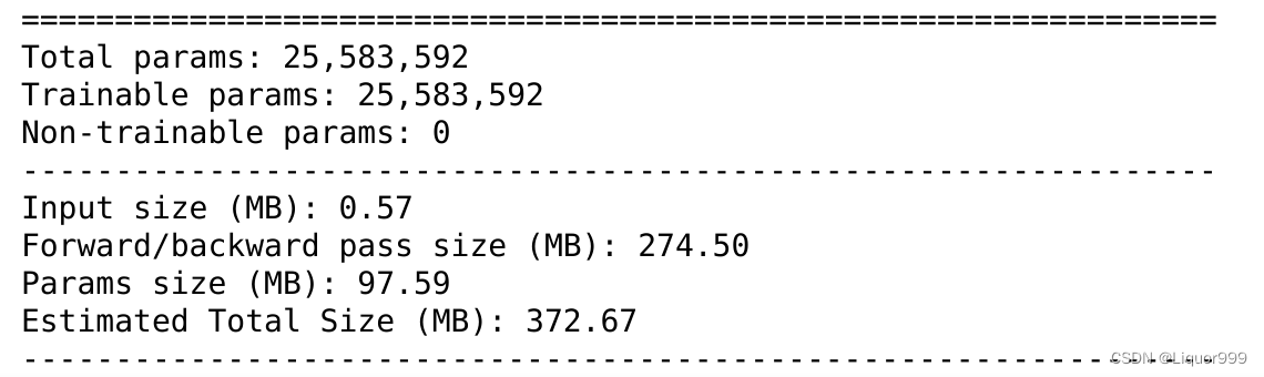
使用summary查看模型架构
from torchsummary import summary
model = ResNet50().to(device)
summary(model, input_size=(3, 224, 224))
开始训练
定义训练函数
def train(dataloader, model, loss_fn, opt):size = len(dataloader.dataset)num_batches = len(dataloader)train_acc, train_loss = 0, 0for X, y in dataloader:X, y = X.to(device), y.to(device)pred = model(X)loss = loss_fn(pred, y)opt.zero_grad()loss.backward()opt.step()train_acc += (pred.argmax(1) == y).type(torch.float).sum().item()train_loss += loss.item()train_acc /= sizetrain_loss /= num_batchesreturn train_acc, train_loss
定义测试函数
def test(dataloader, model, loss_fn):size = len(dataloader.dataset)num_batches = len(dataloader)test_acc, test_loss = 0, 0with torch.no_grad():for X, y in dataloader:X, y = X.to(device), y.to(device)pred = model(X)loss = loss_fn(pred, y)test_acc += (pred.argmax(1) == y).type(torch.float).sum().item()test_loss += loss.item()test_acc /= sizetest_loss /= num_batchesreturn test_acc, test_loss
定义学习率、损失函数、优化算法
loss_fn = nn.CrossEntropyLoss()
learn_rate = 0.00001
opt = torch.optim.Adam(model.parameters(), lr=learn_rate)
开始训练,epoch设置为30
import time
epochs = 30
train_loss = []
train_acc = []
test_loss = []
test_acc = []T1 = time.time()best_acc = 0
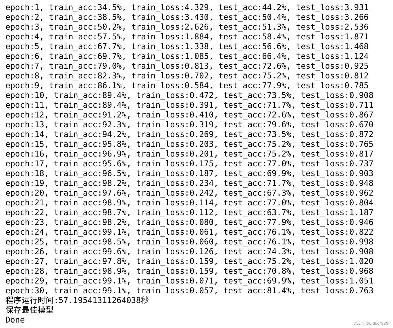
best_model = 0for epoch in range(epochs):model.train()epoch_train_acc, epoch_train_loss = train(train_dl, model, loss_fn, opt)model.eval() # 确保模型不会进行训练操作epoch_test_acc, epoch_test_loss = test(test_dl, model, loss_fn)if epoch_test_acc > best_acc:best_acc = epoch_test_accbest_model = copy.deepcopy(model)train_acc.append(epoch_train_acc)train_loss.append(epoch_train_loss)test_acc.append(epoch_test_acc)test_loss.append(epoch_test_loss)print("epoch:%d, train_acc:%.1f%%, train_loss:%.3f, test_acc:%.1f%%, test_loss:%.3f"% (epoch + 1, epoch_train_acc * 100, epoch_train_loss, epoch_test_acc * 100, epoch_test_loss))T2 = time.time()
print('程序运行时间:%s秒' % (T2 - T1))PATH = './best_model.pth' # 保存的参数文件名
if best_model is not None:torch.save(best_model.state_dict(), PATH)print('保存最佳模型')
print("Done")
结果稍微有些过拟合
可视化
将训练与测试过程可视化
import warnings
warnings.filterwarnings("ignore")               #忽略警告信息
plt.rcParams['font.sans-serif']    = ['SimHei'] # 用来正常显示中文标签
plt.rcParams['axes.unicode_minus'] = False      # 用来正常显示负号
plt.rcParams['figure.dpi']         = 100        #分辨率epochs_range = range(epochs)plt.figure(figsize=(12, 3))
plt.subplot(1, 2, 1)plt.plot(epochs_range, train_acc, label='Training Accuracy')
plt.plot(epochs_range, test_acc, label='Test Accuracy')
plt.legend(loc='lower right')
plt.title('Training and Validation Accuracy')plt.subplot(1, 2, 2)
plt.plot(epochs_range, train_loss, label='Training Loss')
plt.plot(epochs_range, test_loss, label='Test Loss')
plt.legend(loc='upper right')
plt.title('Training and Validation Loss')
plt.show()

模型预测
定义预测函数
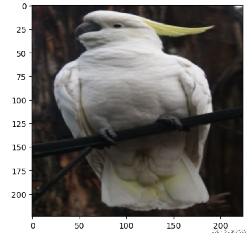
from PIL import Image classes = list(total_data.class_to_idx)def predict_one_image(image_path, model, transform, classes):test_img = Image.open(image_path).convert('RGB')plt.imshow(test_img) # 展示预测的图片test_img = transform(test_img)img = test_img.to(device).unsqueeze(0)model.eval()output = model(img)_,pred = torch.max(output,1)pred_class = classes[pred]print(f'预测结果是:{pred_class}')
开始预测
predict_one_image(image_path='./data/bird_photos/Cockatoo/001.jpg', model=model, transform=all_transforms, classes=classes) # 预测结果是:Cockatoo
总结
本次实验学习了ResNet的基本概念和实现,ResNet的核心思想是通过引入残差块,使网络能够更容易地学习恒等映射的变化部分,所以能够构建深层次的网络, 同时其中的跳跃连接通过将输入直接添加到输出,有助于梯度的流动,减轻梯度消失的问题,但是ResNet计算和存储的资源要求高,容易过拟合也是它的缺点,我们可以通过学习它的网络设计思想,构建自己的网络。