Variance Reduction Methods: a Quick Introduction to Quasi Monte Carlo——完结

https://www.scratchapixel.com/lessons/mathematics-physics-for-computer-graphics/monte-carlo-methods-in-practice/introduction-quasi-monte-carlo
本文主要讲解了，拟蒙特卡洛采样（分层采样、和低差异采样）

u may have heard the term quasi monte carlo or quasi monte carlo ray tracing and wonder what it means (another one of these magic words people from the graphics community use all the time and each time your hear it you grind your teeth in frustration and think “damn if someone could just explain it to me in simple terms”-- that is why we are here for). the math behind quasi monte carlo can be quite complex, and it requires more than a chapter to study them seriously (entire mathematics text books are devoted to the matter). however to give u a complete overview on monte carlo, we wil try in this chapter to give u a quick introduction to this concept, and explain as usual, what it is, how and why it works.

we will revise this chapter, once all other lessons are completed. QMC (Quasi Monte Carlo) is a very interesting method and a lesson will be devoted to this topic in the advanced lesson at some point in time. Once we have completed the lesson on Light Transport Algorithms and Sampling, it will become easier to experiment with QMC and show with more concrete example why it is superior to basic MC.

introduction
basic monte carlo works. we showed this in the previous chapters. it is a great technique, simple to implement and it can be used to solve many problems, especially in computer graphics. we also studied importance sampling in the previous chapter. it potentially reduces variance by increasing the probability of generating samples where the function being integrated is the most important. 通过重要性采样，减少方差。
however both basic monte carlo and important sampling suffer from a problem known as sample clumping. when the samples are generated, some of them might be very close to each other. they form clumps.簇/从
our credit sample being limited we need to use it wisely to gather as much information as possible on the integrand. if two (or more) samples are close to each other, they each provide us the same information on the function (more or less), and thus while one of them is useful the others are definitely wasted. importance sampling does not save us from clumping. the PDF only controls the density of samples within any part of the integrand, not their numbers. and example of clumping is showned in figure 1.

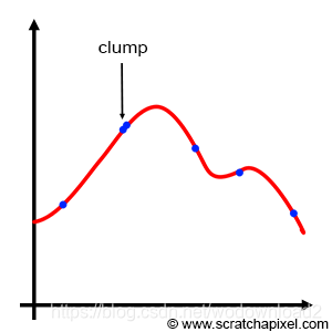
Figure 1: clumping occurs when two or more samples are very close to each other. This can’t be avoided when the position of samples is chosen randomly, even when importance sampling is used.

when Monte Carlo is used, we know that samples are randomly chosen. on the other hand (and in contrast to using a Monte Carlo integration), u can use a deterministic quadratic technique such as the Riemann sum, in which the function is sampled at perfectly regular intervals (as showed in figure 2). so, on one hand we have perfectly regularly spaced samples (with the Riemman sum) and on the other, u have samples whose positions are completely random (with monte carlo integration) which potentially lead to clumping. So, as you may have guessed, you might be tempted to ask: “can we come up with something in between? Can we use some sort of slider to go from completely regularly spaced to completely random, and find some sort of sweet spot somewhere in the middle?” And the quick answer is yes: that’s more or less what Quasi Monte Carlo is all about. Remember that the only reason why we don’t use deterministic techniques such as the Riemann sum is because they don’t scale up well: they become expensive as the dimension of the integral increases. Which is also why MC integration is attractive in comparaison.

in fact, nothing imposes us in a Monte Carlo integration to use stochastic samples. we could very well repalce ξ with a series of evenly distributed samples 均值同分布的in the MC integration, and the resulting estimate would still be valid. in other words, we can replace random samples by non random samples and the approximation still works.

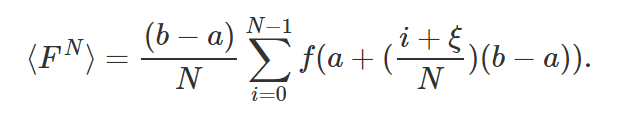
note that when the points are perfectly evenly distributed then, the monte carlo integration and the riemann sum are simiar. if s1, s2, …, sn is a sequence of evenly distributed numbers on the interval [a,b], then:

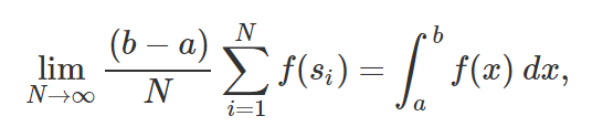
where f is a riemann-integrable function. though in QMC the sequences commonly used are said to be equidistributed, a term we will explain later. but as an intuitive definition, we can say that equidistributed points are points which are more or less evenly distributed, where the measure of the difference the actual point distribution compared to a sequence of points perfectly well distributed is called in QMC jargon术语, discrepancy. in the world of QMC we will not really speak of variance but more of discrepancy. again, these will be explained briefly in this chapter and in more details in the lesson on QMC in the advanced section. but in short, QMC blurs the lines between random and determinisitic sequences. and in effect, the idea behind using these sequences of points, is to get as closely as possible to the ideal situation in which points are well-distributed, and yet not uniformly distributed. Figure 3 below illustrates this idea. The random sequence at the top shows some clumping and gaps (regions with no samples) and thus is not ideal. The sequence in the middle is purely regular and thus will cause aliasing. The sequence at the bottom is somewhere in between: while it exhibits some property of regularity, the points are not completely uniformly distributed. The idea of dividing the sample space into regular intervals and randomly placing a sample within each one of these sub-intervals is called jittering or stratified sampling.

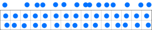
Figure 3: example of randomly distributed samples (top), evenly distributed samples (middle) and “more or less” evenly distributed samples which are typical of what quasi random sequences look like (bottom).

Quasi Monte Carlo methods were first proposed in the 1950s about a decade after Monte Carlo methods (which makes sense because once people started to get familiar with Monte Carlo methods, they started to look into ways of improving them). QMC is used in many areas, engineering, finance and of course computer graphics (to just name a few), and even though few people can claim to be specialists of the subject, it certainly gained popularity over the last few years. Whether using QMC is better than traditional MC in rendering is often debated. It does converge faster than MC bit it has its own disatvantages. For example it can sometimes produce aliasing

Remember that in terms of visual artifact, deterministic techniques such as the Rieman sum produce aliasing while Monte Carlo integration produces noise. Visually noise is often considered as the lesser of two evils, compared to aliasing.

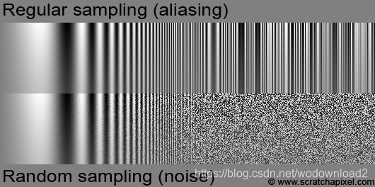
Figure 4: regular sampling (top) produces aliasing while random sampling (bottom) produces noise. Visually, noise is generally less objectionable.

These visual artifact can easily be generated. Figure 4 shows the result of sampling a sine function with increasing frequency. When the sampling rate gets lower than the Nyquist frequency, noise or aliasing show up. A lesson of the advanced of the advanced section is devoted to aliasing in wich the concept of Nyquist limit is explained and we will explain aliasing from a mathematical point of view when we get to the topic of sampling and Fourier analysis (which we kept for the end).

#include <cstdlib> 
#include <cstdio> 
#include <cmath> 
#include <fstream> 
#include <stdint.h> 
 
float evalFunc(const float &x, const float &y, const float &xmax, const float &ymax) 
{ 
    return 1. / 2. + 1. / 2. * powf(1. - y / ymax, 3.) * sin( 2. * M_PI * ( x / xmax) * exp(8. * (x / xmax))); 
} 
 
int main(int argc, char **argv) 
{ 
    uint32_t width = 512, height = 512; 
    uint32_t nsamples = 1; 
    unsigned char *pixels = new unsigned char[width * height]; 
    for (uint32_t y = 0; y < height; ++y) 
    { 
        for (uint32_t x = 0; x < width; ++x) 
        { 
            float sum = 0; 
            for (uint32_t ny = 0; ny < nsamples; ++ny) 
            { 
                for (uint32_t nx = 0; nx < nsamples; ++nx) 
                { 
#ifdef REGULAR //规则的取值
                    sum += evalFunc(x + (nx + 0.5) / nsamples, y + (ny + 0.5) / nsamples, width, height); 
#endif 
#ifdef RANDOM //随机的取值
                    sum += evalFunc(x + drand48(), y + drand48(), width, height); 
#endif 
                } 
            } 
            pixels[y * width + x] = (unsigned char)(255 * sum / (nsamples * nsamples)); 
        } 
    } 
    std::ofstream ofs; 
    ofs.open("./sampling.ppm"); 
    ofs << "P5\n" << width << " " << height << "\n255\n"; 
    ofs.write((char*)pixels, width * height); 
    ofs.close(); 
    delete [] pixels; 
    return 1; 
} 

规则取值会造成锯齿，随机取值会产生噪声。

stratified sampling 分层采样
before we look into generating sequences of quasi random numbers, we will first talk about a method which is somewhere in between random and regular distributed samples. this method is called stratified sampling and was introduced to the graphics community by Robert L. Cook in a seminal 开创性的 paper entitled Stochastic sampling in computer graphics (which he published in 1986 but the technique was developed at pixar in 1983). this paper is quite fundamental to the filed of computer graphics and will be studied in depth in the lesson on sampling (in the basic section). in this paper Cook studied the quality of different sampling strategies notably by using Fourier analysis which is with Monte Carlo theory, another one of these really large topics which we better keep for the end. in his paper, Cook did not call the method stratified sampling but jittered sampling, but nowdays it only seems to be known under the former name. 前

The concept of stratified sampling is very simple. It combines somehow the idea of regular and random sampling. The interval of integration is divided into N subintervals or cells (also often called strata), samples are placed in the middle of these subintervals but are jittered by some negative or positive random offset which can’t be greater than half the width of a cell. In other words if h is the width of the cell: −h/2≤ξ≤h/2. Technically though we generally place the sample on the left boundary of the cell and jitter its position by h∗ξh∗ξ. In other words, we simply place a random sample within each strata. The result can be seen a sum of N Monte Carlo integrals over sub-domains.

extending this idea to 2D is straightforward. the domain of integration (often a unit square, such as pixel for instance) is divided into N*M strata and a random sample is placed within each cell. again, this can easily be extended to higher dimensions. in the case of stratified sampling, variance reduces linearly with the number of samples (σ∝1/N). in almost all cases, stratified sampling is superior to random sampling and should be preferentially used.

quasi random numbers and low-discrepancy sequences
quasi monte carlo integration relies on sequences of points with particular properties. as explained in the introduction, the goal is to generate sequences of samples which are not exactly uniformly distributed (uniform distributed samples can cause aliasing) and yet which appear to have some regularity in the way they are spaced. mathematicians introduced the concept of discrepancy to measure the distribution of these points. intuitively, discrepency can be seen (interpreted) as a measure of how the samples deviate in a way from a regular distribution. random sequences have a high discrepency while a sequence of uniformly distributed samples would have zero discrepancy. the sort of sequences we are after are the ones with the lowest possible discrepancy but not a zero discrepancy. there are sequences which minimize randomness (the deviation of the actual samples position from a uniform distribution should be a small as possible) but are not exactly uniform (i.e. we are obviously not interested not interestd in sequences with 0 discrepancy).

Example: the Van der Corput Sequence

algorithms for generating low discrepancy sequences were found in the 1950’s (it will hopefully be clear to u how computer technology has influenced their design). interestingly, these algorithms are often quite simple to implement (they often only take few lines of code) but the mathematics behind them can be quite complex. these sequences can be generated in different ways but for this introduction we will only consider a particular type of sequence called Van der Corput sequence (many over algorithms are constructed using this approach). having one example to play with, should at lest show u what these sequences look like (and help us to study some of their basic properties). to generate a Van der Corput sequence, u need to be familiar with the concept of radical and radical inverse which we will now explain (we will also explain why it’s called radical inverse further down).

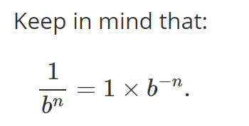
Every integer number can decomposed or redefined if you prefer in a base of your choice. For example our numerical system uses a base ten. Also recall that any number (integer) to the power of zero is one (100=1100=1). So in base 10 for instance, the number 271 could be defined as: 2×10平方 +7×10+1×10^0. Mathematically we could write this sum as:

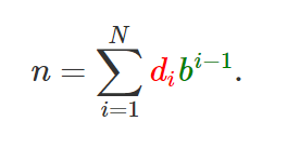
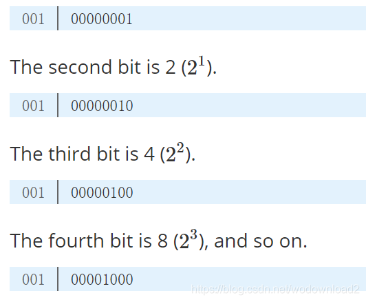
where b is the base in which you want to define your number (in our example b=10) and the d’s which are called digits, are in our example the numbers 2, 7 and 1. The same method can be used with a base two which as you know, is used by computers to encode numbers. The first bit (the one to the right of a byte) represents 1 (2^0).

If you combine these bits together you can create more numbers. For example number 3 can be encoded by turning on the first and second bit. Adding up the numbers they represent gives 3 (20+21=1+2=320+21=1+2=3).

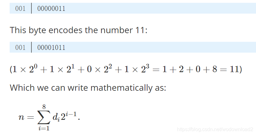
where di in base 2 can either be 0 or 1. With this in hand, we can now decompose any integer into a series of digits in any given base (we call this, a digit expansion in base b). Now note that the number we can recreate with this sequence is a positive integer. In other words, you can see this number as being a series of 0 and 1 on the left inside of a “imaginary” decimal point.

The idea behind the Van der Corput sequence, is to mirror these bits around this imaginary decimal point. For example our number 11, becomes:

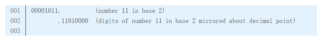
做个镜像反转，上图第二行，是第一行的倒过来。

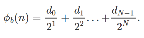
That can be done by making a slight change to the equation which we used for computing n:

乘以底数的幂次。

which is equivalent to:


radical inverse 径向反转

If n = 1 for example,
ϕ2(1)=1×2(-1次方)=0.5 (in base 2).
If n = 3,
ϕ2(3)=1×2(−1次方)+1×2(−2次方)=0.75.
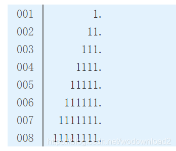
The following table shows the first few numbers of the the Van der Corput sequence (in base 2).

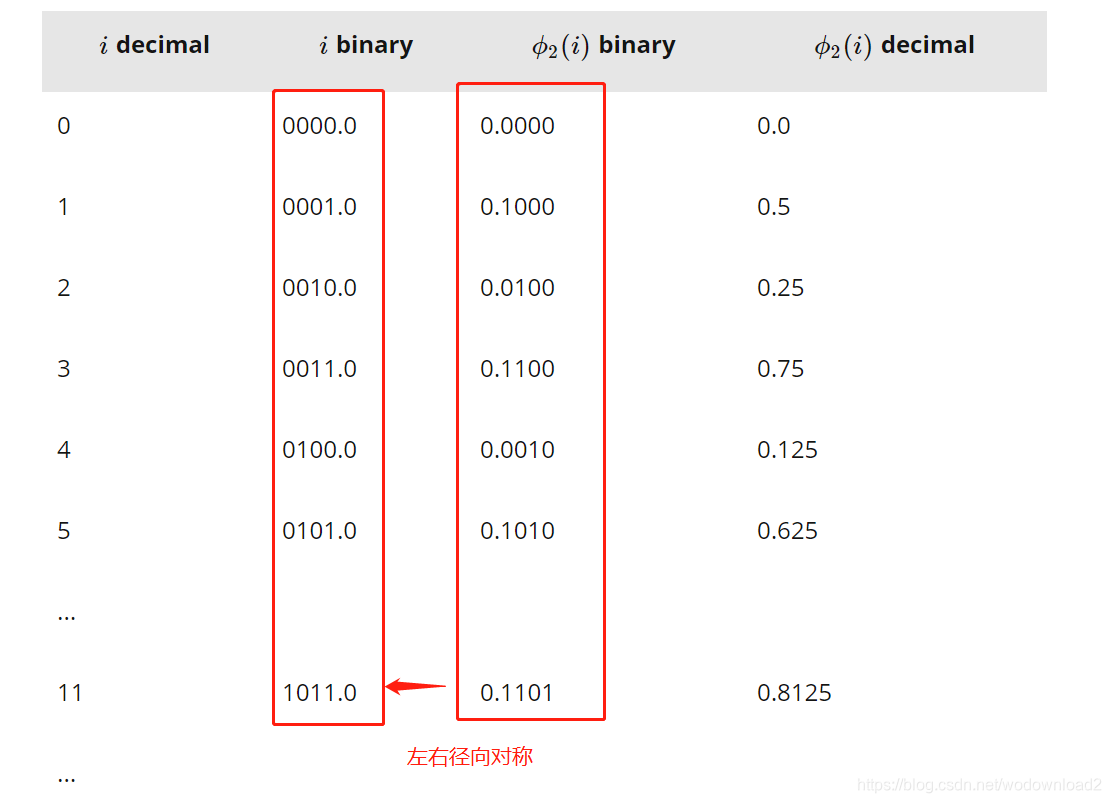
implementing this algorithm is actually quite simple. the first task is to find a way of computing the digit expansion. the function we need is the modulus operator: num%2 computes the remainder when num (an integer) is divided by 2. so for example 1%2 = 0, 2%2=0, 3%2=1, 4%2=0, and son. so in essence num%2 tells us whether the current value of n is a multiple of the base or not. in a binary integer, the only bit that is making the number odd or even is the right-most bit (the least significant bit which has the bit position 0). so if number is even (n%2 = 0), this las bit should be 0.

int n = 11; 
int base = 2; 
int d0 = n % base; // it returns either 0 or 1 

the next step is to start adding up the result of the digit divided by the base raised to the power of the digit position plus one (as in equation 1).

int n = 11; 
float result = 0; 
int base = 2; 
int d0 = n % base; // it returns either 0 or 1 
int denominator = base; // 2 = powf(base, 1) 
result += d0 / denominator;

Finally here is the complete implementation of the algorithm:

#include <iostream> 
#include <cmath> 
 
float vanDerCorput(int n, const int &base = 2) 
{ 
    float rand = 0, denom = 1, invBase = 1.f / base; 
    while (n) { 
        denom *= base; // 2, 4, 8, 16, etc, 2^1, 2^2, 2^3, 2^4 etc. 
        rand += (n % base) / denom; 
        n *= invBase; // divide by 2 
    } 
    return rand; 
} 
 
int main() 
{ 
    for (int i = 0; i < 10; ++i) { 
        float r = vanDerCorput(i, 2); 
        printf("i %d, r = %f\n", i, r); 
    } 
    return 0; 
} 

the van der corput sequence has been extended to multi-dimensions by Halton (1960), Sobel (1967), Faure (1982) and Niederreiter (1987). for more information, check the lesson on Sampling in the advanced section. https://www.scratchapixel.com/lessons/mathematics-physics-for-computer-graphics/monte-carlo-methods-in-practice/introduction-quasi-monte-carlo

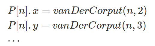
the Halton sequence uses different van der corput sequences in different bases, where the base is a prime number (2,3,5,7,11, etc,). for example if u want to generate 2D points, u can assign a van der corput sequence in base 2 to the x coordinates of the points, and another sequence in base 3 to the point’s y coordinate.

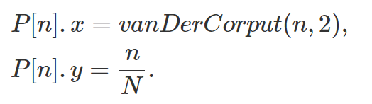
the hammersley sequence uses a van der corput sequence in base 2 for one of the coordinates and just assign n/N to the other (assuming your point is a 2D point). //这里的第二维度只是用n/N

the following code creats an Halton sequence for generating 2D points:

#include <iostream> 
#include <cmath> 
 
float vanDerCorput(int n, const int &base = 2) 
{ 
   ... 
} 
 
int main() 
{ 
    Point2D pt; 
    for (int i = 0; i < 10; ++i) { 
        pt.x = vanDerCorput(i, 2); // prime number 2 
        pt.x = vanDerCorput(i, 3); // prime number 3 
        printf("i %d, pt.x = %f pt.y\n", i, pt.x, pt.y); 
    } 
    return 0; 
} 

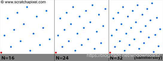
the figure above shows a plot of points from a 2D Hammersely sequence for different number of samples (N=16, 24 and 32). note that the point (0,0) in red, is always in the sequence 0点是一直有的，and that points are nicely distributed for all values of N. 所有的点分布的都很好。the code used to generated the Van der Corput sequence can be optimized using bit operations (for instance dividing a integer by 2 can be done with a bit shift operation). because the sequence is called with incrementing values of n, results of previous calculation could also be re-used n的增大，但是前面的计算结果是可以重用的。 (which could also speed up the generation of the samples). the next revision of this lesson will include an optimized version of this function.

quasi monte carlo
the idea behind quasi monte carlo is obviously to use quasi random sequences in the generation of samples rather than random samples. these sequences are very often used to generate pixel samples. In this lesson and the lesson Introduction to Shading and Radiometry, we showed how Monte Carlo integration could be used to approximate radiance passing through a given pixel (figure 7). Random sampling is of course the easiest (at least the most basic) way of generating these samples. We can also use stratified sampling (which is better than random sampling) or of course quasi random sequences (like the Halton or the Hammersley sequence which we talked about in this chapter). When low-discrepancy sequences are used, we speak of Quasi Monte Carlo ray tracing (as opposed to Monte Carlo ray tracing which is using random or stratified sampling). Note that computing the radiance of a pixel is only one example of Monte Carlo integration in which low-discrepancy sequences can be used. Halton, Hammersley or any other such sequences are also commonly used in shading (this will be explained in the next lessons).

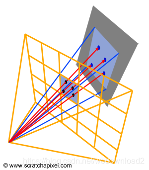
Figure 7: using Monte Carlo integration to approximate radiance passing through a given pixel.

Pros and Cons of Stratified Sampling & Quasi Monte Carlo
QMC has a faster rate of convergence than random sampling and this is certainly its main advantages from a rendering point of view (we will explain mathematically why in a future revision of revision of this lesson). Images produced with low-discrepancy sequences, have generally less noise and have a better visual quality than images produced with random sampling (for the sample number of samples). With stratified sampling it is not always possible to efficiently generate samples for arbitrary values of N (try to generate 7 2D samples for instance using stratified sampling) while with low-discrepancy sequences, this is not a problem. Furthermore, note that if you want to change the value of N, you can do so without losing the previously calculated samples. N can be increased while all samples from the earlier computation can still be used. This is particularly useful in adaptive algorithms in which typically a low number of samples is used as a starting point and more samples are generated on the fly in areas of the frame where variance is high.

Cons: as mentioned earlier in this chapter, QMC can suffer from aliasing and more over, because low-discrepancy have a periodic structure, they can generate a discernible明显的 pattern (figure 8). This is particularly hard to avoid as sequences are potentially re-used from one pixel to another. Getting rid of the structure can require additional work (such as rotating the samples, etc.).
This potentially makes a robust implementation of LDS in a renderer more complex than the stratified sampling approach which is really simple to implement.
QMC 拟蒙特卡洛 has been been a quite active field of research since the 2000’s. While low discrepancy sequences are now considered as a viable 可行的替代方案 alternative to other sampling methods, there is still an active debate in the graphics community as whether they are superior to other methods and really worth the pain. A. Kensler for instance, has recently published a new technique for generating stratified samples which is competitive with low discrepancy quasi-Monte Carlo sequences (see reference below).

Generally, generating (good) random sequences is a complex art and studying their properties involved complex techniques (such as Fourier analysis). A chapter can only give a very superficial 肤浅的 overview of these methods. You will find a more thorough 彻底的 treatment 治疗方案 of the subject matter in this lesson on sampling which you can find in the advanced section.

Figure 8: the periodic structure of some low-discrepancy sequences can sometimes be clearly visible. © Leonhard Grünschloß

A Final World
This conclude our introduction to Monte Carlo methods. These lessons hopefully gave you a good understanding of what Monte Carlo methods are, how and why they work. While we spoke about Monte Carlo ray tracing a few times in the last few lessons, you may still want to see how all the things we learned so far apply to rendering and ray tracing in particular. This is the topic of our next lesson.

Reference
Stochastic Sampling in Computer Graphics, Robert L. Cook, Siggraph 1986.
Efficient Multidimensional Sampling, T. Kollig and A. Keller, 2002.
Correlated Multi-Jittered Sampling, A. Kensler, 2013.