当前位置：首页 > news >正文

【Python深度学习】Python全栈体系（三十三）

news 来源：原创 2024/5/3 1:08:22

深度学习

第十四章 PaddlePaddle 概览

一、PaddlePaddle 简介

1. 什么是 PaddlePaddle ？

PaddlePaddle （Parallel Distributed Deep Learning，中文名飞桨）是百度公司推出的开源，易学习，易使用的分布式深度学习平台
源于产业实践，在实际中有着优异表现
支持多种机器学习经典模型

2. 为什么学习 PaddlePaddle？

开源，国产
提供算力支持，能完成复杂的图像任务
程序简洁，使用较为简单，降低教学和学习难度

3. PaddlePaddle 优点

易用性。语法简介，API的设计干净清晰
丰富的模型库。借助于其丰富的模型库，可以非常容易的复现一些经典方法
全中文说明文档。首家完整支持中文文档的深度学习平台
运行速度快。充分利用 GPU 集群的性能，为分布式环境的并行计算进行加速

4. PaddlePaddle 缺点

教材少
行业应用较少

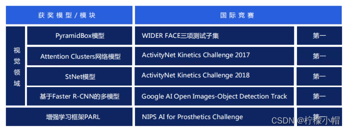
5. 国际竞赛获奖情况

在这里插入图片描述

6. 行业应用

在这里插入图片描述

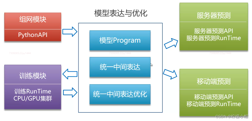
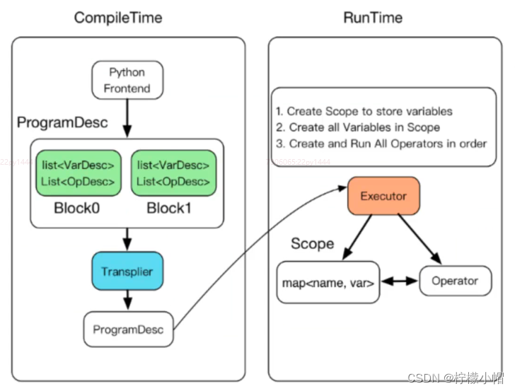
二、体系结构

1. 总体架构

在这里插入图片描述

2. 编译时与执行时

在这里插入图片描述

3. 三个重要术语

Fluid：定义程序执行流程
Program：对用户来说是一个完整的程序
Executor：执行器，执行程序

4. 代码

在这里插入图片描述

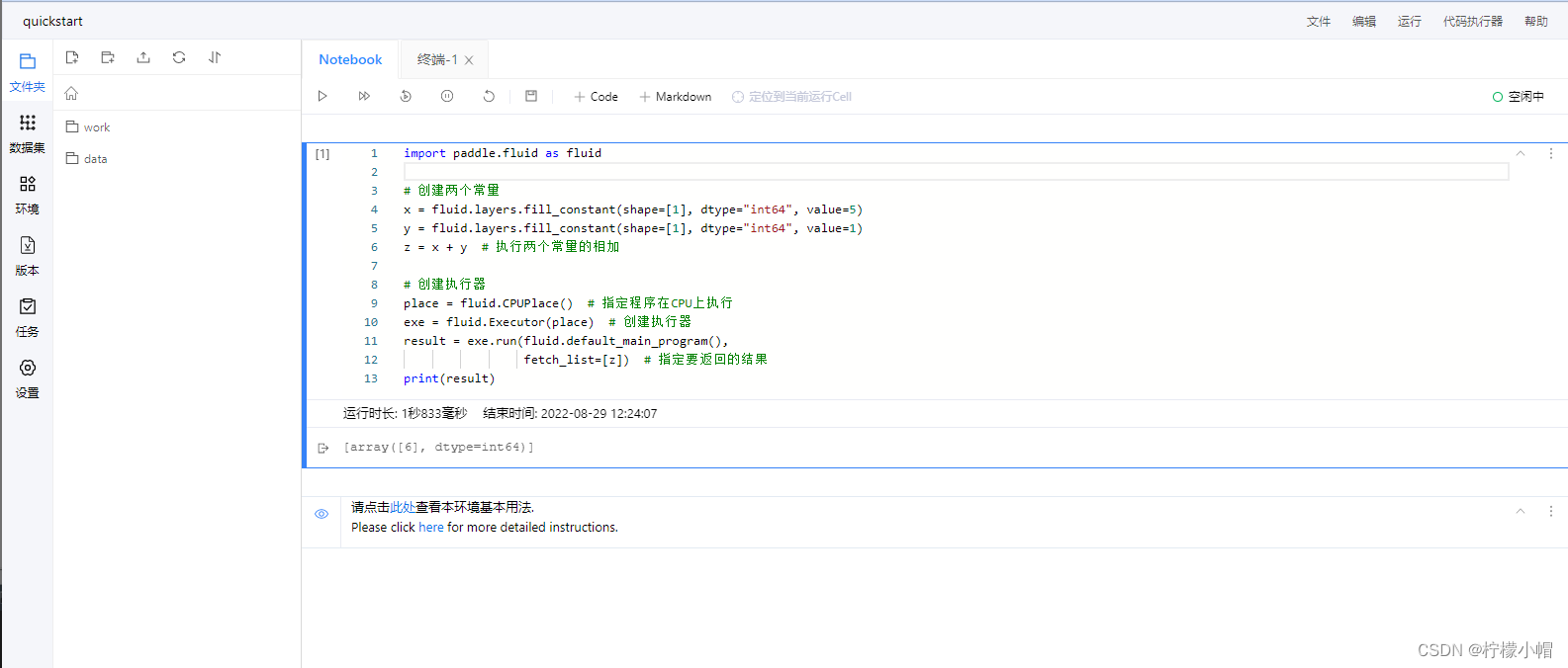
# paddlepaddle版本：1.5
import paddle.fluid as fluid

# 创建两个常量
x = fluid.layers.fill_constant(shape=[1], dtype="int64", value=5)
y = fluid.layers.fill_constant(shape=[1], dtype="int64", value=1)
z = x + y  # 执行两个常量的相加

# 创建执行器
place = fluid.CPUPlace()  # 指定程序在CPU上执行
exe = fluid.Executor(place)  # 创建执行器
result = exe.run(fluid.default_main_program(),
                 fetch_list=[z])  # 指定要返回的结果
print(result)
"""
[array([6], dtype=int64)]
"""

第十五章基本概念与操作

基本概念

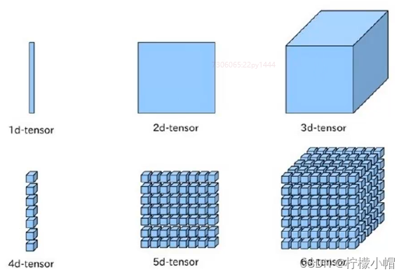
1. 张量

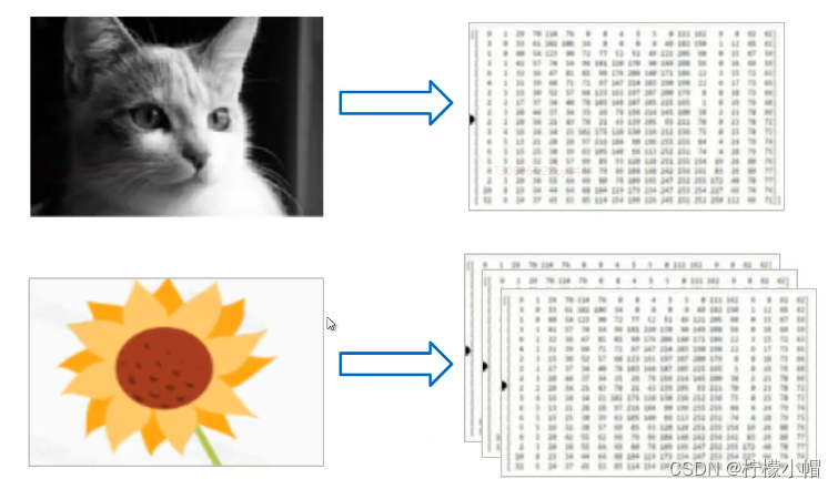
张量（Tensor）：多维数组或向量，同其它主流深度学习框架一样，PaddlePaddle使用张量来承载数据
灰度图像为二维张量（矩阵），彩色图像为三维张量

2. Layer

表示一个独立的计算逻辑，通常包含一个或多个operator（操作），如layers.relu表示ReLU计算；layers.pool2d表示pool操作。Layer的输入和输出为Variable。

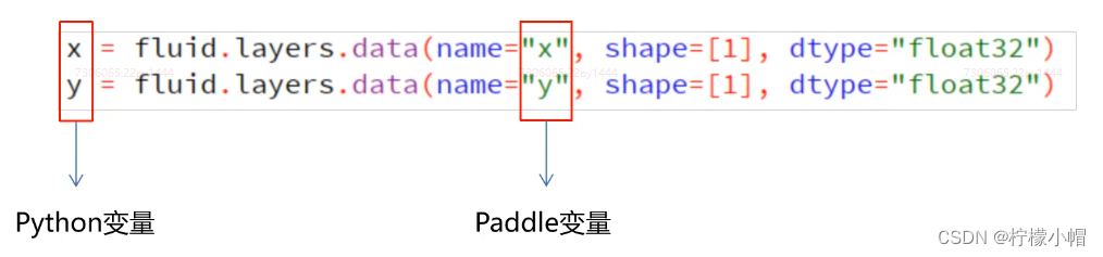
3. Variable

表示一个变量，可以是一个张量（Tensor），也可以是其它类型。Variable进入Layer计算，然后Layer返回Variable。创建变量方式：

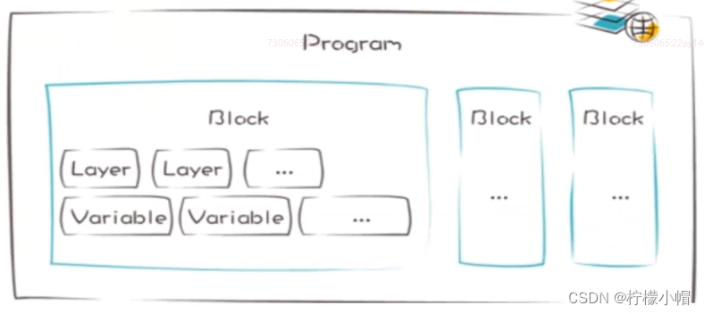
4. Program

Program包含Variable定义的多个变量和Layer定义的多个计算，是一套完整的计算逻辑。从用户角度来看，Program是顺序、完整执行的。

5. Executor

Executor用来接收并执行Program，会一次执行Program中定义的所有计算。通过feed来传入参数，通过fetch_list来获取执行结果。

outs = exe.run(fluid.default_main_program(), # 默认程序上执行
			   feed=params, # 喂入参数
			   fetch_list=[result]) # 获取结果

6. Place

PaddlePaddle 可以运行在Intel CPU，Nvidia GPU，ARM CPU和更多嵌入式设备上，可以通过Place用来指定执行的设备（CPU或GPU）。

place = fluid.CPUPlace() 	 # 指定CPU执行
place = fluid.CUDAPlace(0) 	 # 指定GPU执行

7. Optimizer

优化器，用于优化网络，一般用来对损失函数做梯度下降优化，从而求得最小损失值

8. 代码

# 变量（张量）示例
import paddle.fluid as fluid
import numpy

# 创建两个变量，2行3列，类型为浮点型
x = fluid.layers.data(name="x", shape=[2, 3], dtype="float32")
y = fluid.layers.data(name="y", shape=[2, 3], dtype="float32")

x_add_y = fluid.layers.elementwise_add(x, y)  # 张量按元素相加
x_mul_y = fluid.layers.elementwise_mul(x, y)  # 张量按元素相乘

place = fluid.CPUPlace()  # 指定在CPU上执行
exe = fluid.Executor(place)  # 执行器
exe.run(fluid.default_startup_program())  # 初始化

a = numpy.array([[1, 2, 3],
                 [4, 5, 6]])
b = numpy.array([[1, 1, 1],
                 [2, 2, 2]])
params = {"x": a, "y": b}  # 参数字典
outs = exe.run(program=fluid.default_main_program(),  # 要执行的program
               feed=params,  # 执行program需要的参数
               fetch_list=[x_add_y, x_mul_y])  # 指定要获取的结果
print(numpy.array(outs).shape)
for i in outs:
    print(i)

"""
(2, 2, 3)
[[2 3 4]
 [6 7 8]]
[[ 1  2  3]
 [ 8 10 12]]
"""

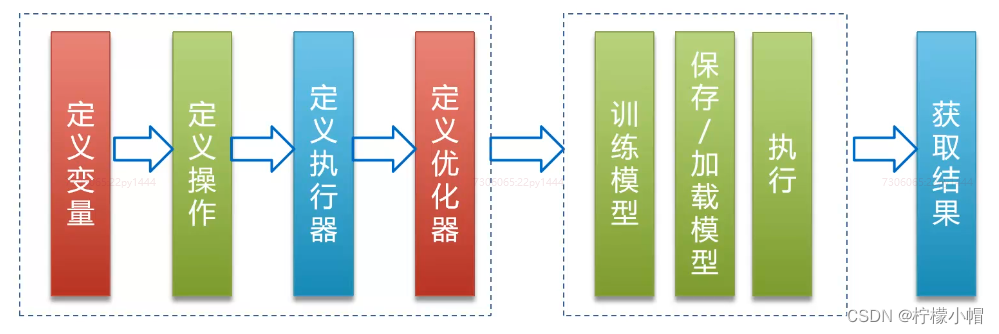
9. 程序执行步骤

在这里插入图片描述

第十六章综合案例：实现线性回归

线性回归

1. 案例3：编写简单线性回归

在这里插入图片描述

2. 代码

# 简单线性回归
import paddle
import paddle.fluid as fluid
import numpy as np
import matplotlib.pyplot as plt

# 定义样本
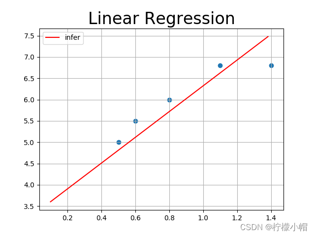
train_data = np.array([[0.5], [0.6], [0.8], [1.1], [1.4]]).astype("float32")
y_true = np.array([[5.0], [5.5], [6.0], [6.8], [6.8]]).astype("float32")

# 定义变量
x = fluid.layers.data(name="x", shape=[1], dtype="float32")
y = fluid.layers.data(name="y", shape=[1], dtype="float32")

# 搭建模型，构建损失函数，优化器
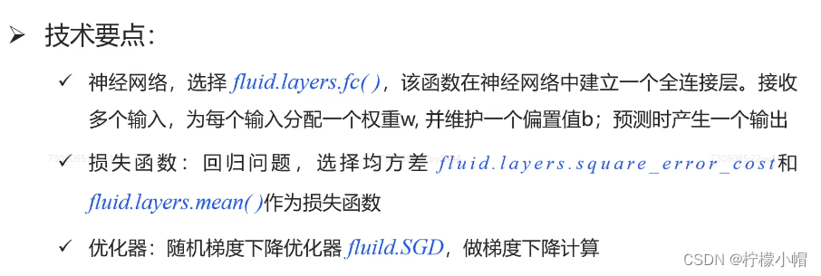
y_predict = fluid.layers.fc(input=x,  # 输入数据
                            size=1,  # 输出值的个数
                            act=None)  # 激活函数，回归这里不采用激活函数

# 损失函数
cost = fluid.layers.square_error_cost(input=y_predict,  # 预测值
                               label=y)  # 真实值
avg_cost = fluid.layers.mean(cost) # 均方差
# 优化器
optimizer = fluid.optimizer.SGD(learning_rate=0.01) # 随机梯度下降优化器
optimizer.minimize(avg_cost) # 指定要优化的对象

# 执行器
place = fluid.CPUPlace()
exe = fluid.Executor(place)
exe.run(fluid.default_startup_program())

# 开始迭代训练
costs = []
iters = []
params = {"x":train_data, "y":y_true} # 参数字典

for i in range(200):
    outs = exe.run(feed=params, # 传入的参数
                   fetch_list=[y_predict.name, avg_cost.name])
    iters.append(i) # 记录迭代次数
    costs.append(outs[1][0]) # 记录损失值
    print("i: ", i, "cost: ", outs[1][0])

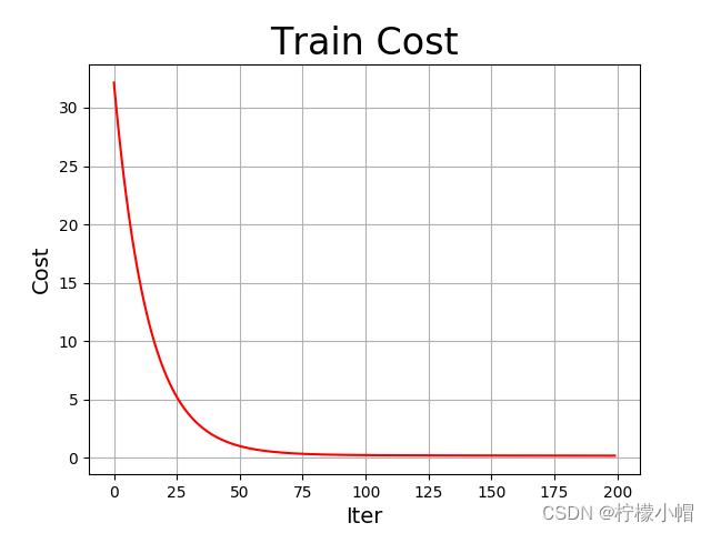
# 损失函数可视化
plt.figure("Training")
plt.title("Train Cost", fontsize=24)
plt.xlabel("Iter", fontsize=14)
plt.ylabel("Cost", fontsize=14)
plt.plot(iters, costs, color="red", label="Train Cost")
plt.grid()
plt.savefig("train.png") # 保存图片

# 线性模型可视化
tmp = np.random.rand(10, 1) # 生成10行1列的均匀的随机数组
tmp = tmp * 2 # 范围放大
tmp.sort(axis=0) # 排序
x_test = np.array(tmp).astype("float32")
params = {"x":x_test, "y":x_test} # y不参加计算，仅仅是为了避免语法错误
y_out = exe.run(feed=params,
                fetch_list=[y_predict.name]) # 返回预测结果
y_test = y_out[0]

plt.figure("Infer")
plt.title("Linear Regression", fontsize=24)
plt.plot(x_test, y_test, color="red", label="infer")
plt.scatter(train_data, y_true) # 绘制原始样本散点图

plt.legend()
plt.grid()
plt.savefig("infer.png")
plt.show()

"""
i:  0 cost:  32.14875
i:  1 cost:  29.862375
i:  2 cost:  27.739735
i:  3 cost:  25.769098
i:  4 cost:  23.939585
i:  5 cost:  22.24108
i:  6 cost:  20.664204
i:  7 cost:  19.200241
i:  8 cost:  17.841106
i:  9 cost:  16.579292
i:  10 cost:  15.4078245
i:  11 cost:  14.320238
i:  12 cost:  13.310519
i:  13 cost:  12.373095
i:  14 cost:  11.502786
i:  15 cost:  10.694782
i:  16 cost:  9.944625
i:  17 cost:  9.24817
i:  18 cost:  8.601569
i:  19 cost:  8.001253
i:  20 cost:  7.4439073
i:  21 cost:  6.9264526
i:  22 cost:  6.4460325
i:  23 cost:  5.999995
i:  24 cost:  5.5858774
i:  25 cost:  5.201392
i:  26 cost:  4.8444185
i:  27 cost:  4.5129848
i:  28 cost:  4.2052617
i:  29 cost:  3.9195523
i:  30 cost:  3.6542792
i:  31 cost:  3.4079788
i:  32 cost:  3.1792922
i:  33 cost:  2.9669576
i:  34 cost:  2.7698038
i:  35 cost:  2.5867443
i:  36 cost:  2.4167686
i:  37 cost:  2.2589402
i:  38 cost:  2.112389
i:  39 cost:  1.9763073
i:  40 cost:  1.8499448
i:  41 cost:  1.7326069
i:  42 cost:  1.6236455
i:  43 cost:  1.5224622
i:  44 cost:  1.4284992
i:  45 cost:  1.341239
i:  46 cost:  1.2602023
i:  47 cost:  1.1849433
i:  48 cost:  1.1150477
i:  49 cost:  1.0501318
i:  50 cost:  0.9898391
i:  51 cost:  0.9338385
i:  52 cost:  0.88182247
i:  53 cost:  0.8335059
i:  54 cost:  0.7886235
i:  55 cost:  0.74693
i:  56 cost:  0.7081963
i:  57 cost:  0.672211
i:  58 cost:  0.63877684
i:  59 cost:  0.60771143
i:  60 cost:  0.5788453
i:  61 cost:  0.5520208
i:  62 cost:  0.5270917
i:  63 cost:  0.5039226
i:  64 cost:  0.48238698
i:  65 cost:  0.46236864
i:  66 cost:  0.44375867
i:  67 cost:  0.42645583
i:  68 cost:  0.41036686
i:  69 cost:  0.39540488
i:  70 cost:  0.38148916
i:  71 cost:  0.36854538
i:  72 cost:  0.35650307
i:  73 cost:  0.34529853
i:  74 cost:  0.3348711
i:  75 cost:  0.3251656
i:  76 cost:  0.31613076
i:  77 cost:  0.30771756
i:  78 cost:  0.2998822
i:  79 cost:  0.29258323
i:  80 cost:  0.2857826
i:  81 cost:  0.27944416
i:  82 cost:  0.27353522
i:  83 cost:  0.268025
i:  84 cost:  0.2628848
i:  85 cost:  0.2580886
i:  86 cost:  0.25361156
i:  87 cost:  0.24943061
i:  88 cost:  0.24552512
i:  89 cost:  0.24187514
i:  90 cost:  0.2384623
i:  91 cost:  0.23526998
i:  92 cost:  0.23228231
i:  93 cost:  0.22948468
i:  94 cost:  0.22686367
i:  95 cost:  0.2244062
i:  96 cost:  0.22210129
i:  97 cost:  0.21993744
i:  98 cost:  0.21790509
i:  99 cost:  0.2159946
i:  100 cost:  0.21419752
i:  101 cost:  0.21250553
i:  102 cost:  0.2109113
i:  103 cost:  0.20940804
i:  104 cost:  0.20798898
i:  105 cost:  0.20664816
i:  106 cost:  0.20538029
i:  107 cost:  0.20417997
i:  108 cost:  0.20304254
i:  109 cost:  0.20196381
i:  110 cost:  0.20093882
i:  111 cost:  0.19996476
i:  112 cost:  0.19903736
i:  113 cost:  0.19815376
i:  114 cost:  0.1973104
i:  115 cost:  0.19650479
i:  116 cost:  0.19573417
i:  117 cost:  0.19499631
i:  118 cost:  0.19428857
i:  119 cost:  0.19360924
i:  120 cost:  0.1929558
i:  121 cost:  0.19232717
i:  122 cost:  0.19172087
i:  123 cost:  0.19113576
i:  124 cost:  0.19057044
i:  125 cost:  0.19002345
i:  126 cost:  0.18949324
i:  127 cost:  0.18897915
i:  128 cost:  0.1884798
i:  129 cost:  0.18799429
i:  130 cost:  0.18752147
i:  131 cost:  0.18706083
i:  132 cost:  0.18661138
i:  133 cost:  0.18617228
i:  134 cost:  0.18574297
i:  135 cost:  0.18532269
i:  136 cost:  0.18491097
i:  137 cost:  0.18450731
i:  138 cost:  0.18411079
i:  139 cost:  0.18372127
i:  140 cost:  0.18333833
i:  141 cost:  0.18296146
i:  142 cost:  0.18259028
i:  143 cost:  0.18222466
i:  144 cost:  0.18186378
i:  145 cost:  0.1815077
i:  146 cost:  0.18115589
i:  147 cost:  0.18080838
i:  148 cost:  0.18046463
i:  149 cost:  0.18012469
i:  150 cost:  0.17978814
i:  151 cost:  0.17945506
i:  152 cost:  0.17912471
i:  153 cost:  0.17879744
i:  154 cost:  0.17847298
i:  155 cost:  0.17815109
i:  156 cost:  0.17783158
i:  157 cost:  0.17751442
i:  158 cost:  0.17719956
i:  159 cost:  0.17688681
i:  160 cost:  0.17657606
i:  161 cost:  0.1762673
i:  162 cost:  0.17596017
i:  163 cost:  0.17565484
i:  164 cost:  0.17535129
i:  165 cost:  0.17504928
i:  166 cost:  0.17474873
i:  167 cost:  0.17444973
i:  168 cost:  0.1741523
i:  169 cost:  0.17385599
i:  170 cost:  0.17356104
i:  171 cost:  0.17326745
i:  172 cost:  0.17297497
i:  173 cost:  0.17268378
i:  174 cost:  0.17239359
i:  175 cost:  0.17210452
i:  176 cost:  0.17181674
i:  177 cost:  0.1715299
i:  178 cost:  0.1712438
i:  179 cost:  0.17095914
i:  180 cost:  0.17067508
i:  181 cost:  0.17039225
i:  182 cost:  0.17010994
i:  183 cost:  0.16982885
i:  184 cost:  0.16954863
i:  185 cost:  0.1692693
i:  186 cost:  0.16899088
i:  187 cost:  0.16871312
i:  188 cost:  0.16843624
i:  189 cost:  0.16816023
i:  190 cost:  0.16788514
i:  191 cost:  0.16761053
i:  192 cost:  0.16733672
i:  193 cost:  0.16706398
i:  194 cost:  0.16679177
i:  195 cost:  0.16652039
i:  196 cost:  0.1662497
i:  197 cost:  0.16597958
i:  198 cost:  0.16571043
i:  199 cost:  0.16544196
<Figure size 640x480 with 1 Axes>
<Figure size 640x480 with 1 Axes>
"""