当前位置：首页 > news >正文

Machine learning week 10(Andrew Ng)

news 来源：原创 2024/5/8 15:58:15

文章目录

- Reinforcement learning
- - 1. Reinforcement learning introduction
  - - 1.1. What is Reinforcement Learning?
    - 1.2. Mars rover example
    - 1.3. The return in Reinforcement learning
    - 1.4. Making decisions: Policies in reinforcement learning
    - 1.5. Review of key concepts
  - 2. State-action value function
  - - 2.1. State-action value function definition
    - 2.2. State-action value function example
    - 2.3. Bellman Equation
    - 2.4. Random (stochastic) environment
  - 3. Continuous state spaces
  - - 3.1. Example of continuous state space applications
    - 3.2. Lunar lander
    - 3.3. Learning the state-value function
    - 3.4. Algorithm refinement: Improved neural network architecture
    - 3.5. Algorithm refinement: ε-greedy policy
    - 3.6. Algorithm refinement: Mini-batch and soft update
    - 3.7. The state of reinforcement learning
- Summary

Reinforcement learning

1. Reinforcement learning introduction

1.1. What is Reinforcement Learning?

The key idea is rather than you need to tell the algorithm what the right output y for every single input is, all you have to do instead is specify a reward function that tells it when it’s doing well and when it’s doing poorly.

1.2. Mars rover example

1.3. The return in Reinforcement learning

在这里插入图片描述
The first step is $r^0$ .

Select the orientation according to the first two tables

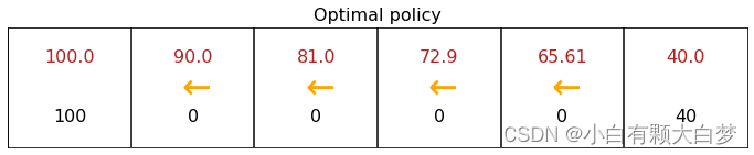
1.4. Making decisions: Policies in reinforcement learning

For example, $\pi(2)$ is left while $\pi(5)$ is right. The number expresses state.
在这里插入图片描述

1.5. Review of key concepts

在这里插入图片描述

2. State-action value function

2.1. State-action value function definition

在这里插入图片描述
The iteration will be used.

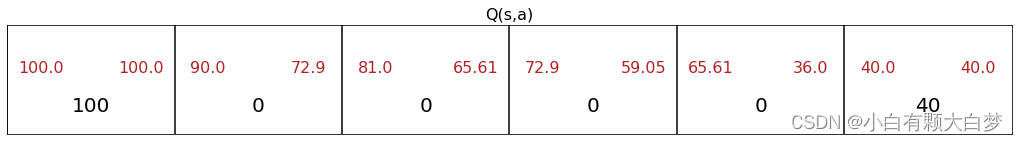
2.2. State-action value function example

2.3. Bellman Equation

$Q(s,a) = R(s) + r * max Q(s^{'},a^{'})$
在这里插入图片描述

2.4. Random (stochastic) environment

Sometimes it actually ends up accidentally slipping and going in the opposite direction.

3. Continuous state spaces

3.1. Example of continuous state space applications

Every variable is continuous.

3.2. Lunar lander

在这里插入图片描述

3.3. Learning the state-value function

在这里插入图片描述

Q is a random value at first. We will train the model to find a better Q.

3.4. Algorithm refinement: Improved neural network architecture

在这里插入图片描述

3.5. Algorithm refinement: ε-greedy policy

ε = 0.05
在这里插入图片描述
If we choose a bad ε, we may take 100 times as long.

3.6. Algorithm refinement: Mini-batch and soft update

The idea of mini-batch gradient descent is to not use all 100 million training examples on every single iteration through this loop. Instead, we may pick a smaller number, let me call it m prime equals say, 1,000. On every step, instead of using all 100 million examples, we would pick some subset of 1,000 or m prime examples.
在这里插入图片描述

Soft update
When we set Q equals to $Q_{new}$ , it can make a very abrupt change to Q.So we will adjust the parameters in Q.
$W = 0.01*W_{new} + 0.99 W$
$B = 0.01*B_{new} + 0.99 B$