1.导入

import numpy as np
import matplotlib.pyplot as plt
from utils import *
import copy
import math

%matplotlib inline

2.逻辑回归

在这部分练习中，你将建立一个逻辑回归模型来预测学生是否被大学录取。

2.1 问题陈述

假设你是一所大学系的管理员，你想根据两次考试的结果来确定每个申请人的入学机会。

• 您有以前申请者的历史数据，可以用作逻辑回归的培训集。

• 对于每个培训示例，您都有申请人在两次考试中的分数以及录取决定。

• 你的任务是建立一个分类模型，根据这两门考试的分数估计申请者的录取概率。

2.2 数据加载和可视化

您将从加载此任务的数据集开始。

• 下面显示的load_dataset（）函数将数据加载到变量X_train和y_train中
• X_train包含学生两次考试的成绩
• “y_train”是录取决定
• y_train=1如果学生被录取
• y_train=0如果学生未被录取
• X_train和`y_train’都是numpy数组。

加载数据

# load dataset
X_train, y_train = load_data("data/ex2data1.txt")

熟悉一下数据集

print("First five elements in X_train are:\n", X_train[:5]) #查看前五条数据
print("Type of X_train:",type(X_train))


First five elements in X_train are:
 [[34.62365962 78.02469282]
 [30.28671077 43.89499752]
 [35.84740877 72.90219803]
 [60.18259939 86.3085521 ]
 [79.03273605 75.34437644]]
Type of X_train: <class 'numpy.ndarray'>

print("First five elements in y_train are:\n", y_train[:5])
print("Type of y_train:",type(y_train))

First five elements in y_train are:
 [0. 0. 0. 1. 1.]
Type of y_train: <class 'numpy.ndarray'>

print ('The shape of X_train is: ' + str(X_train.shape))
print ('The shape of y_train is: ' + str(y_train.shape))
print ('We have m = %d training examples' % (len(y_train)))

The shape of X_train is: (100, 2)
The shape of y_train is: (100,)
We have m = 100 training examples

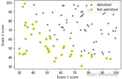
数据可视化

# Plot examples
plot_data(X_train, y_train[:], pos_label="Admitted", neg_label="Not admitted")

# Set the y-axis label
plt.ylabel('Exam 2 score') 
# Set the x-axis label
plt.xlabel('Exam 1 score') 
plt.legend(loc="upper right")
plt.show()

2.3 Sigmoid函数

$$f_{\mathbf{w},b}(x)=g(\mathbf{w}\cdot \mathbf{x}+b)$$

$$g(z)=\frac{1}{1+e^{-z}}$$

Exercise 1

Please complete the sigmoid function to calculate

$$g(z)=\frac{1}{1+e^{-z}}$$

Note that

• z 不一定是一个数，也可以是一个数组
• 如果输入时数组，要对每个sigmoid函数应用值
• 记得np.exp()的使用

def sigmoid(z):
    """
    Compute the sigmoid of z

    Args:
        z (ndarray): A scalar, numpy array of any size.

    Returns:
        g (ndarray): sigmoid(z), with the same shape as z
         
    """
    g = 1/(1+(np.exp(-z)))
    
    return g

2.4 逻辑回归的代价函数 Cost function for logistic regression

Exercise 2

Please complete the compute_cost function using the equations below.

Recall that for logistic regression, the cost function is of the form

$$J(\mathbf{w},b)=\frac{1}{m}\sum _{i=0}^{m-1}\left[loss(f_{\mathbf{w},b}({\mathbf{x}}^{(i)}),y^{(i)})\right]\text{\hspace{1em}(1)}$$

where

• m is the number of training examples in the dataset

• $loss(f_{\mathbf{w},b}({\mathbf{x}}^{(i)}),y^{(i)})$ is the cost for a single data point, which is -

  $$loss(f_{\mathbf{w},b}({\mathbf{x}}^{(i)}),y^{(i)})=(-y^{(i)}\log \left(f_{\mathbf{w},b}\left({\mathbf{x}}^{(i)}\right)\right)-\left(1-y^{(i)}\right)\log \left(1-f_{\mathbf{w},b}\left({\mathbf{x}}^{(i)}\right)\right)\text{\hspace{1em}(2)}$$

• $f_{\mathbf{w},b}({\mathbf{x}}^{(i)})$ is the model’s prediction, while $y^{(i)}$, which is the actual label

• $f_{\mathbf{w},b}({\mathbf{x}}^{(i)})=g(\mathbf{w}\cdot {\mathbf{x}}^{(\mathbf{i})}+b)$ where function $g$ is the sigmoid function.

  • It might be helpful to first calculate an intermediate variable $z_{\mathbf{w},b}({\mathbf{x}}^{(i)})=\mathbf{w}\cdot {\mathbf{x}}^{(\mathbf{i})}+b=w_0{x}_0^{(i)}+...+w_{n-1}{x}_{n-1}^{(i)}+b$ where $n$ is the number of features, before calculating $f_{\mathbf{w},b}({\mathbf{x}}^{(i)})=g(z_{\mathbf{w},b}({\mathbf{x}}^{(i)}))$

Note:

• As you are doing this, remember that the variables X_train and y_train are not scalar values but matrices of shape ($m,n$) and ($m$,1) respectively, where $n$ is the number of features and $m$ is the number of training examples.
• You can use the sigmoid function that you implemented above for this part.
• numpy有np.log()

def compute_cost(X, y, w, b, lambda_= 1):
    """
    Computes the cost over all examples
    Args:
      X : (ndarray Shape (m,n)) data, m examples by n features
      y : (array_like Shape (m,)) target value 
      w : (array_like Shape (n,)) Values of parameters of the model      
      b : scalar Values of bias parameter of the model
      lambda_: unused placeholder
    Returns:
      total_cost: (scalar)         cost 
    """

    m, n = X.shape
    loss_sum = 0
    ### START CODE HERE ###
    for i in range(m):
      z_wb = 0
      for j in range(n):
        z_wb_xi = w[j] * X[i][j]
        z_wb += z_wb_xi

      z_wb += b
      f_wb = sigmoid(z_wb)
      loss = -y[i] * np.log(f_wb) - (1-y[i]) * np.log(1-f_wb)
      loss_sum += loss

    total_cost = loss_sum/m
    ### END CODE HERE ### 
    
    return total_cost

代码测试

m, n = X_train.shape

# Compute and display cost with w initialized to zeroes
initial_w = np.zeros(n)
initial_b = 0.
cost = compute_cost(X_train, y_train, initial_w, initial_b)
print('Cost at initial w (zeros): {:.3f}'.format(cost))

Cost at initial w (zeros): 0.693

2.5 逻辑回归的梯度下降