机器学习笔记-线性回归
机器学习笔记
- 线性回归
- K-邻近算法/KNN-API
- 距离度量
- 交叉验证法,k的值选取
- 鸢尾花数据集API
- 鸢尾花数据集数据可视化API
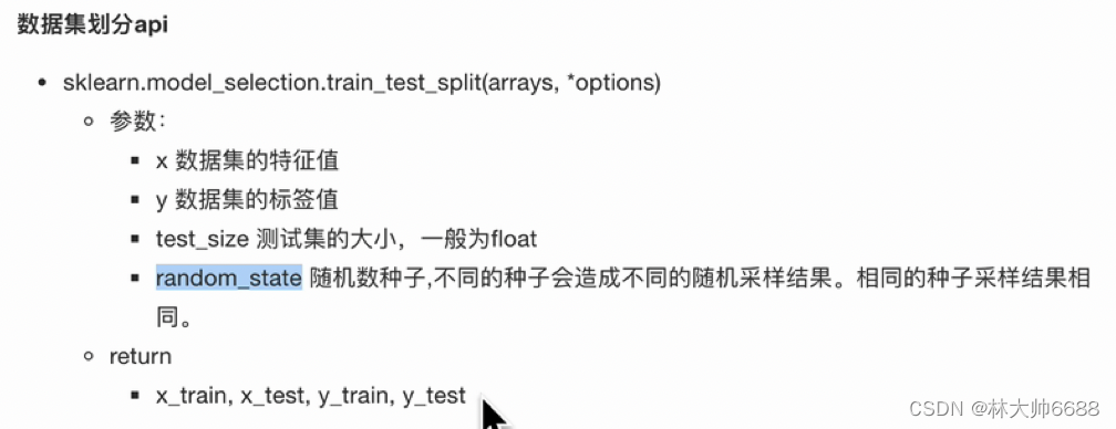
- 鸢尾花数据集划分API
- 特征工程与处理API
- 归一化
- 标准化
- 再识K-邻近算法API
- API总结
- 归一化的API
- 标准化API
- 交叉验证API
- 线性回归-API
- 损失函数
- 优化损失函数 正规方程
- 优化损失函数 梯度下降
- 梯度下降各种类别
- 回归性能分析
- 欠拟合和过拟合
- 解决过拟合
- 解决过拟合-岭回归(和梯度下降一样)
- 解决过拟合-Lasso回归
- 解决过拟合-弹性网络
- 解决过拟合-早停
- 模型的保存和加载
线性回归
K-邻近算法/KNN-API
from sklearn.neighbors import KNeighborsClassifier

# 1.构造数据
x = [[1], [2], [3], [4]]
y = [0, 1, 2, 3]

# 2.训练模型
# 2.1 实例化一个估计器对象;这里的n_neighbors一般为5.取1个邻近样本
estimator = KNeighborsClassifier(n_neighbors=1)

# 2.2 调用fit方法,进行训练
estimator.fit(x, y)

# 3.数据预测
ret = estimator.predict([[0.1]])
print(ret)#结果为0;因为邻近x的4所以,y是y[3]=1;
# 可以这样理解, x是特征值, 是dataframe形式理解为二维的[[]],
# y表示的目标值, 可以表示为series, 表示为一维数组[]
ret1 = estimator.predict([[2.52]])
print(ret1)#结果为1;因为邻近x的4所以,y是y[3]=1;
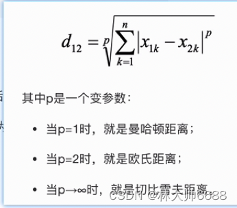
距离度量
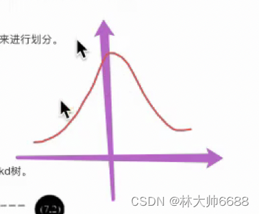
交叉验证法,k的值选取
- 背景知识,方差越小,越瘦高,数据越集中;方差越大数据越分散是最好的。
鸢尾花数据集API
from sklearn.datasets import load_iris

# 1.数据集获取
# 1.1 小数据集获取
iris = load_iris()
# print(iris)

# 1.2 大数据集获取
# news = fetch_20newsgroups()
# print(news)

# 2.数据集属性描述
print("数据集特征值是:\n", iris.data)
print("数据集目标值是:\n", iris["target"])
print("数据集的特征值名字是:\n", iris.feature_names)
print("数据集的目标值名字是:\n", iris.target_names)
print("数据集的描述:\n", iris.DESCR)
鸢尾花数据集数据可视化API
import seaborn as sns
import matplotlib.pyplot as plt
import pandas as pd
from sklearn.datasets import load_iris, fetch_20newsgroups
from sklearn.model_selection import train_test_split
# 1.数据集获取
# 1.1 小数据集获取
iris = load_iris()
# 3.数据可视化
iris_d = pd.DataFrame(data=iris.data, columns=['Sepal_Length', 'Sepal_Width', 'Petal_Length', 'Petal_Width'])
iris_d["target"] = iris.target
print(iris_d)
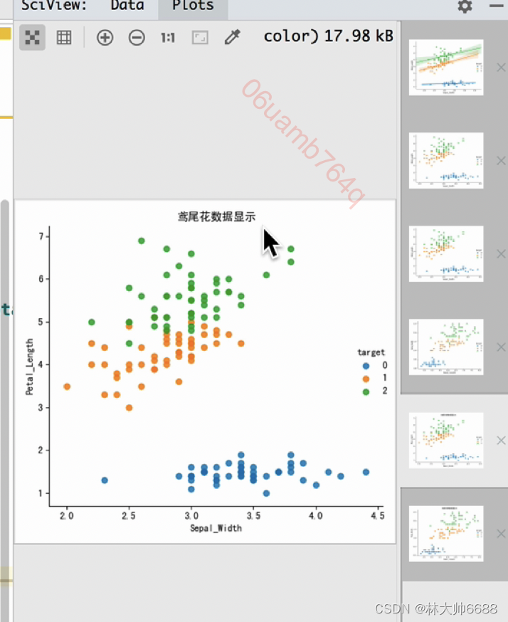
def iris_plot(data, col1, col2):
sns.lmplot(x=col1, y=col2, data=data, hue="target", fit_reg=False)
plt.title("鸢尾花数据显示")
plt.rcParams['font.sans-serif'] = ['SimHei']
plt.rcParams['axes.unicode_minus'] = False
plt.show()
iris_plot(iris_d, 'Sepal_Width', 'Petal_Length')
iris_plot(iris_d, 'Sepal_Length', 'Petal_Width')
鸢尾花数据集划分API
特征工程与处理API
归一化
-
公式

-
直接在jupyter中运行即可,注意read_csv
import pandas as pd
from sklearn.preprocessing import MinMaxScaler, StandardScaler
def minmax_demo():
"""
归一化演示
:return:None
"""
data = pd.read_csv("./data/dating.txt")
print(data)
# 1.实例化
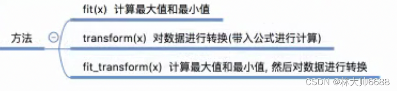
transfer = MinMaxScaler(feature_range=(3,5))
# 2.进行转换, 调用fit_transform
ret_data = transfer.fit_transform(data[["milage", "Liters", "Consumtime"]])
print("归一化之后的数据为:\n",ret_data)
minmax_demo()
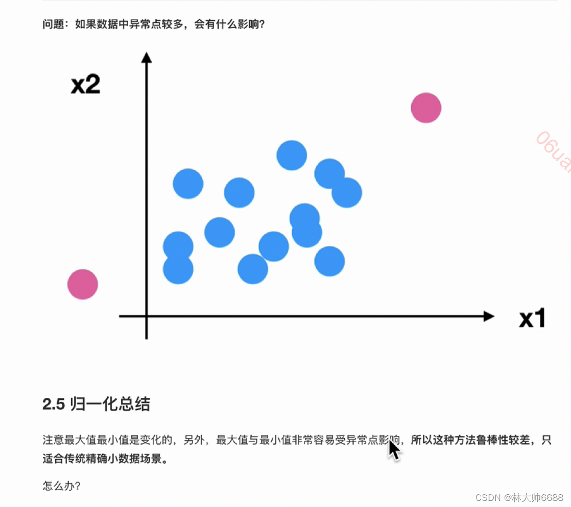
- 鲁棒性(确定性、稳定性):就是归一化后容易收到异常值的影响,归一化的鲁棒性就差容易收到异常值的影响;归一化只适合小数据集的;
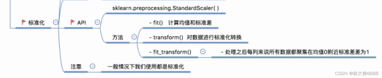
标准化
- 公式

import pandas as pd
from sklearn.preprocessing import MinMaxScaler, StandardScaler

def stand_demo():
    """
    标准化演示
    :return:None
    """
    data = pd.read_csv("./data/dating.txt")
    print(data)

    # 1.实例化
    transfer = StandardScaler()

    # 2.进行转换, 调用fit_transform
    ret_data = transfer.fit_transform(data[["milage", "Liters", "Consumtime"]])
    print("标准化之后的数据为:\n",ret_data)
    print("每一列的方差为:\n", transfer.var_)
    print("每一列的平均值为:\n", transfer.mean_)

stand_demo()
再识K-邻近算法API
from sklearn.datasets import load_iris# 1.获取数据
from sklearn.model_selection import train_test_split# 2.数据基本处理
from sklearn.preprocessing import StandardScaler# 3.标准化
from sklearn.neighbors import KNeighborsClassifier# 4.机器学习-KNN

# 1.获取数据
iris = load_iris()

# 2.数据基本处理-数据的划分,分成训练和测试集
x_train, x_test, y_train, y_test = train_test_split(iris.data, iris.target, test_size=0.2, random_state=22)

# 3.特征工程 - 特征预处理
transfer = StandardScaler()
x_train = transfer.fit_transform(x_train)
x_test = transfer.transform(x_test)

# 4.机器学习-KNN
# 4.1 实例化一个估计器
estimator = KNeighborsClassifier(n_neighbors=5)
# 4.2 模型训练
estimator.fit(x_train, y_train)

# 5.模型评估
# 5.1 预测值结果输出
y_pre = estimator.predict(x_test)
print("预测值是:\n", y_pre)
print("预测值和真实值的对比是:\n", y_pre==y_test)

# 5.2 准确率计算
score = estimator.score(x_test, y_test)
print("准确率为:\n", score)
API总结
归一化的API
标准化API
交叉验证API
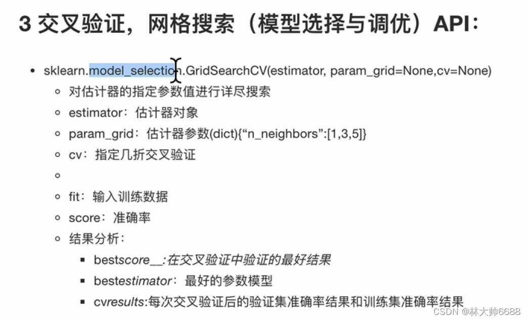
from sklearn.datasets import load_iris
from sklearn.model_selection import train_test_split, GridSearchCV
from sklearn.preprocessing import StandardScaler
from sklearn.neighbors import KNeighborsClassifier

# 1.获取数据
iris = load_iris()

# 2.数据基本处理
x_train, x_test, y_train, y_test = train_test_split(iris.data, iris.target, test_size=0.2, random_state=22)

# 3.特征工程 - 特征预处理
transfer = StandardScaler()
x_train = transfer.fit_transform(x_train)
x_test = transfer.transform(x_test)

# 4.机器学习-KNN
# 4.1 实例化一个估计器
estimator = KNeighborsClassifier()

# 4.2 模型调优 -- 交叉验证,网格搜索
param_grid = {"n_neighbors": [1, 3, 5, 7]}
estimator = GridSearchCV(estimator, param_grid=param_grid, cv=5)

# 4.3 模型训练
estimator.fit(x_train, y_train)

# 5.模型评估
# 5.1 预测值结果输出
y_pre = estimator.predict(x_test)
print("预测值是:\n", y_pre)
print("预测值和真实值的对比是:\n", y_pre == y_test)

# 5.2 准确率计算
score = estimator.score(x_test, y_test)
print("准确率为:\n", score)

# 5.3 查看交叉验证,网格搜索的一些属性
print("在交叉验证中,得到的最好结果是:\n", estimator.best_score_)
print("在交叉验证中,得到的最好的模型是:\n", estimator.best_estimator_)
print("在交叉验证中,得到的模型结果是:\n", estimator.cv_results_)

- 解释,交叉验证只能提高可信度;网格搜索才能提高准确度。

线性回归-API

- API

损失函数
- 公式(又称为最小二乘法);优化方法正规方程和梯度下降。其实就是把损失函数的值降到最低。


优化损失函数 正规方程
求解例子

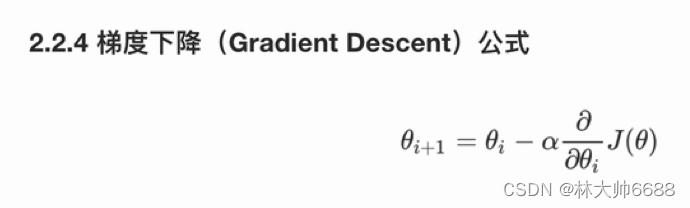
优化损失函数 梯度下降
- α就是步长或者叫学习率

- 例子

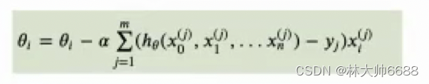
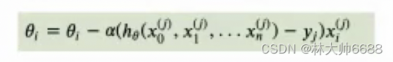
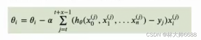
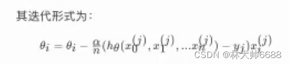
梯度下降各种类别
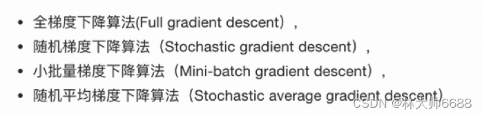
-
全梯度下降公式
-
随机梯度下降公式
-
小批量梯度下降公式
-
随机平均梯度下降公式
回归性能分析

# coding:utf-8

"""
# 1.获取数据
# 2.数据基本处理
# 2.1 分割数据
# 3.特征工程-标准化
# 4.机器学习-线性回归
# 5.模型评估
"""

from sklearn.datasets import load_boston
from sklearn.model_selection import train_test_split
from sklearn.preprocessing import StandardScaler
from sklearn.linear_model import LinearRegression, SGDRegressor, RidgeCV, Ridge
from sklearn.metrics import mean_squared_error


def linear_model1():
    """
    线性回归:正规方程
    :return:
    """
    # 1.获取数据
    boston = load_boston()
    # print(boston)

    # 2.数据基本处理
    # 2.1 分割数据
    x_train, x_test, y_train, y_test = train_test_split(boston.data, boston.target, test_size=0.2)

    # 3.特征工程-标准化
    transfer = StandardScaler()
    x_train = transfer.fit_transform(x_train)
    x_test = transfer.fit_transform(x_test)

    # 4.机器学习-线性回归
    estimator = LinearRegression()
    estimator.fit(x_train, y_train)

    print("这个模型的偏置是:\n", estimator.intercept_)
    print("这个模型的系数是:\n", estimator.coef_)

    # 5.模型评估
    # 5.1 预测值
    y_pre = estimator.predict(x_test)
    # print("预测值是:\n", y_pre)

    # 5.2 均方误差
    ret = mean_squared_error(y_test, y_pre)
    print("均方误差:\n", ret)


def linear_model2():
    """
    线性回归:梯度下降法
    :return:
    """
    # 1.获取数据
    boston = load_boston()
    # print(boston)

    # 2.数据基本处理
    # 2.1 分割数据
    x_train, x_test, y_train, y_test = train_test_split(boston.data, boston.target, test_size=0.2)

    # 3.特征工程-标准化
    transfer = StandardScaler()
    x_train = transfer.fit_transform(x_train)
    x_test = transfer.fit_transform(x_test)

    # 4.机器学习-线性回归
    # estimator = SGDRegressor(max_iter=1000, learning_rate="constant", eta0=0.001)
    estimator = SGDRegressor(max_iter=1000)
    estimator.fit(x_train, y_train)

    print("这个模型的偏置是:\n", estimator.intercept_)
    print("这个模型的系数是:\n", estimator.coef_)

    # 5.模型评估
    # 5.1 预测值
    y_pre = estimator.predict(x_test)
    # print("预测值是:\n", y_pre)

    # 5.2 均方误差
    ret = mean_squared_error(y_test, y_pre)
    print("均方误差:\n", ret)


def linear_model3():
    """
    线性回归:岭回归
    :return:None
    """
    # 1.获取数据
    boston = load_boston()
    # print(boston)

    # 2.数据基本处理
    # 2.1 分割数据
    x_train, x_test, y_train, y_test = train_test_split(boston.data, boston.target, test_size=0.2)

    # 3.特征工程-标准化
    transfer = StandardScaler()
    x_train = transfer.fit_transform(x_train)
    x_test = transfer.fit_transform(x_test)

    # 4.机器学习-线性回归 solver一般默认是SGD随机梯度下降
    # estimator = Ridge(alpha=1.0)
    estimator = RidgeCV(alphas=(0.001, 0.01, 0.1, 1, 10, 100))
    estimator.fit(x_train, y_train)

    print("这个模型的偏置是:\n", estimator.intercept_)
    print("这个模型的系数是:\n", estimator.coef_)

    # 5.模型评估
    # 5.1 预测值
    y_pre = estimator.predict(x_test)
    # print("预测值是:\n", y_pre)

    # 5.2 均方误差
    ret = mean_squared_error(y_test, y_pre)
    print("均方误差:\n", ret)


if __name__ == '__main__':
    linear_model1() #线性回归:正规方程
    linear_model2() #线性回归:梯度下降法
    linear_model3() #线性回归:岭回归
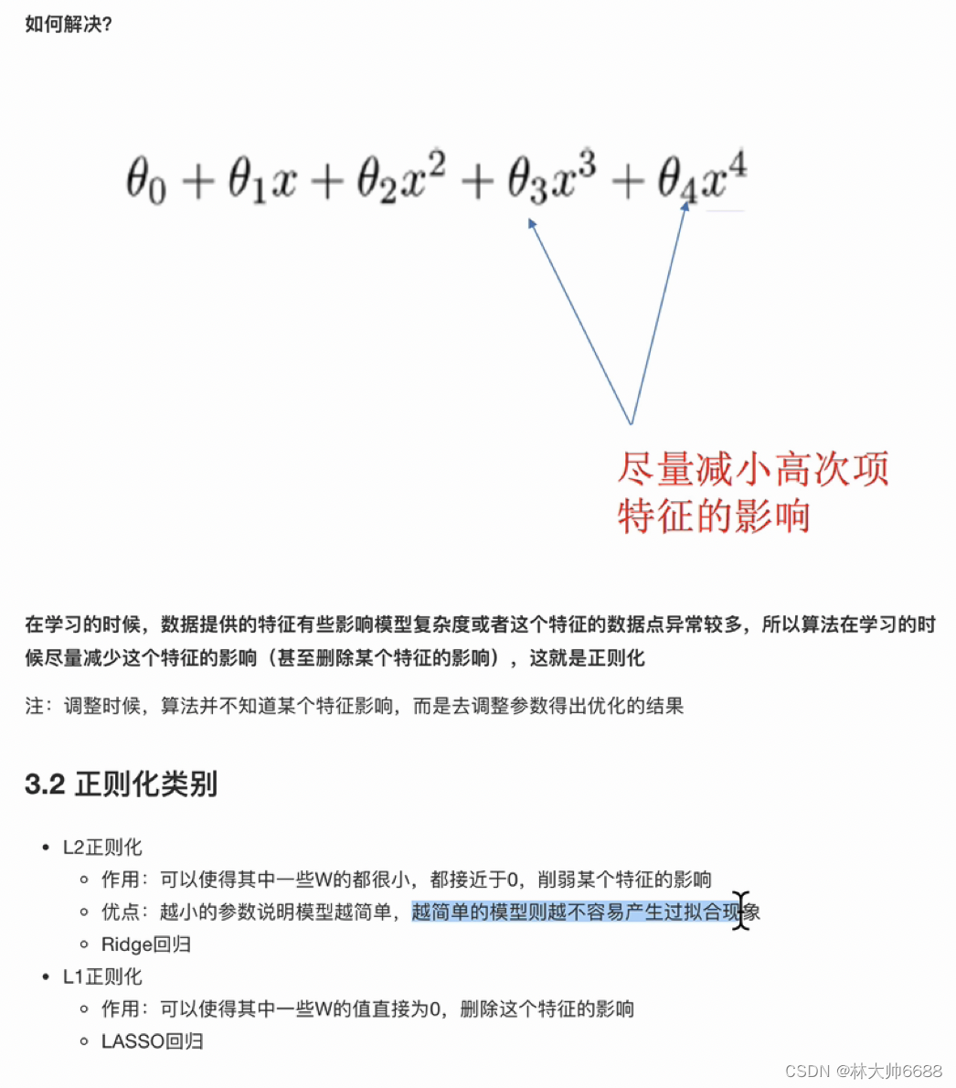
欠拟合和过拟合

解决过拟合
-
综述

-
正则化,一般是参数alpha。

-
L1正则化3,4项直接为0;L2正则化:3,4项无限接近0。
解决过拟合-岭回归(和梯度下降一样)
- 岭回归公式(加的是L2正则项)
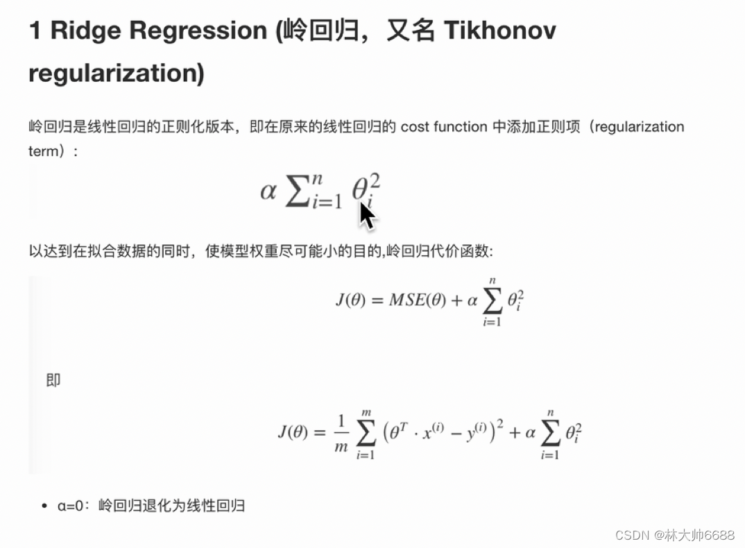
- API

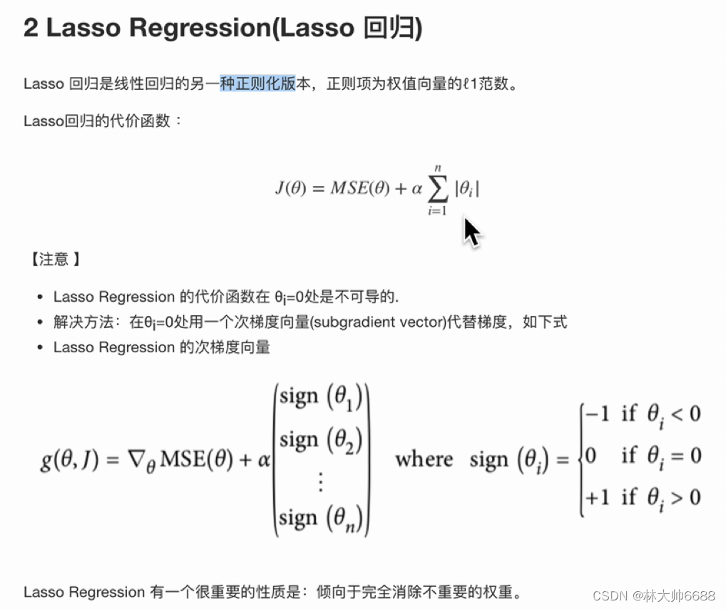
解决过拟合-Lasso回归
- Lasso回归公式(加的是L1正则项)
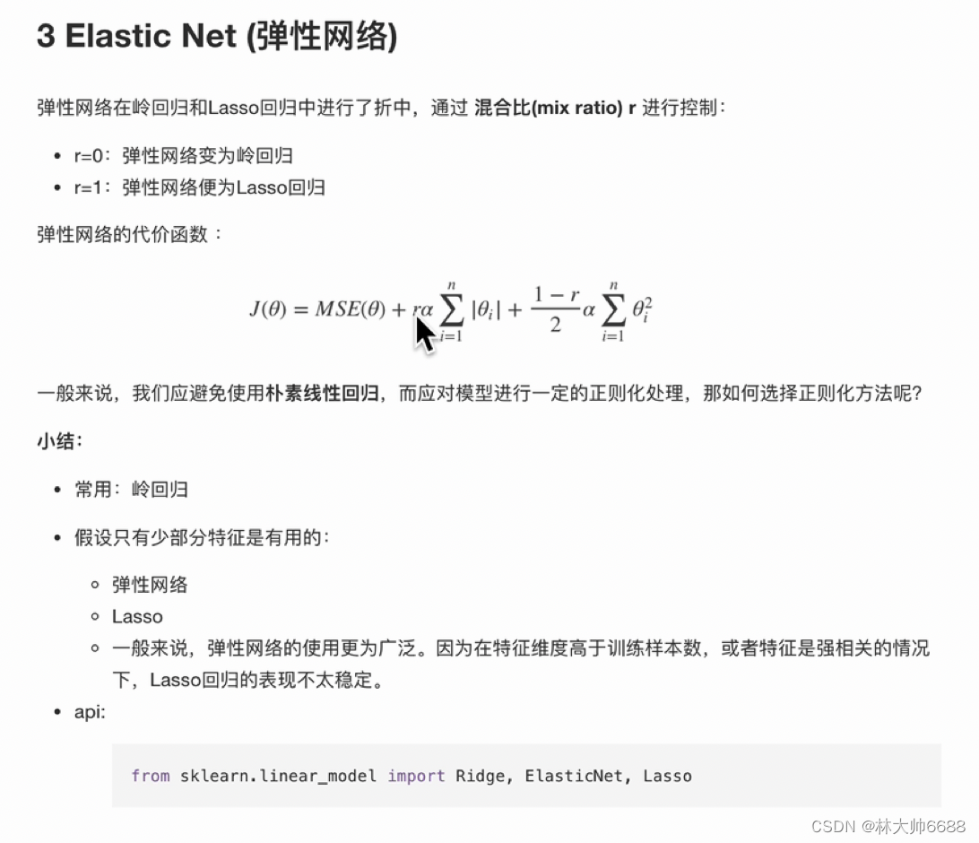
解决过拟合-弹性网络
- 弹性网络(可以在L1和L2中切换,主要看r)
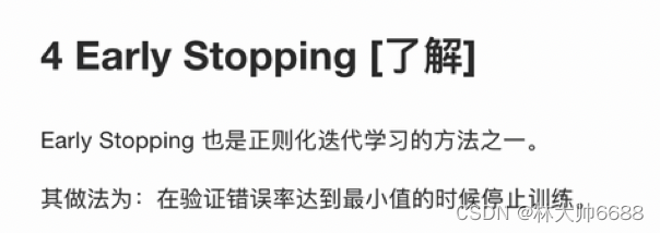
解决过拟合-早停
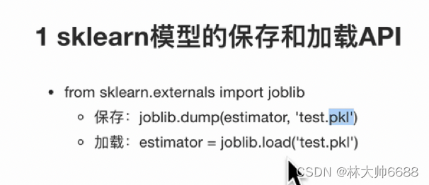
模型的保存和加载