【机器学习】Linear Regression Experiment 线性回归实验 + Python代码实现
文章目录
- 一、实验目标分析
- 1.1 主要实验内容
- 1.2 回归方程复习
- 1.3 构造数据集
- 二、参数直接求解方法
- 2.1 在数据集加上全为1的一列(偏置项)
- 2.2 根据公式求最佳theta值
- 2.3 可视化回归线
- 2.4 sklearn实现线性回归
- 三、常用预处理方法
- 3.1 归一化
- 3.2 标准化
- 3.3 中心化
- 3.4 预处理方法小结
- 四、梯度下降模块
- 4.1 全批量梯度下降
- 4.2 随机梯度下降
- 4.3 MiniBatch小批量随机梯度下降
- 4.4 不同梯度下降策略对比
- 五、多项式回归
- 5.1 构造复杂数据集
- 5.2 多项式特征提取+线性回归求解
- 5.3 拟合曲线可视化
- 5.4 不同多项式拟合效果对比
- 六、样本数量对结果的影响
- 七、正则化
- 7.1 观察过拟合的现象
- 7.2 两种正则化
- 7.2.1 岭回归正则化
- 7.2.2 Lasso回归正则化
一、实验目标分析
1.1 主要实验内容
- 线性回归方程实现
- 梯度下降效果
- 对比不同稀度下降策略
- 建模曲线分析
- 过拟合与欠拟合
- 正则化的作用
- 提前停止策略
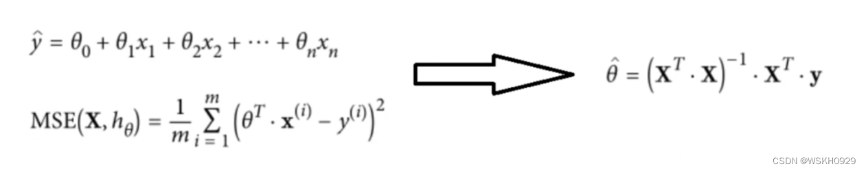
1.2 回归方程复习
1.3 构造数据集
# 构造数据集
import numpy as np

X = 2 * np.random.rand(100, 1)
y = 4 + 3 * X + np.random.randn(100, 1)

plt.plot(X,y,'bo')
plt.xlabel('$x$')
plt.ylabel('$y$')
plt.grid()
plt.show()

二、参数直接求解方法
2.1 在数据集加上全为1的一列(偏置项)
X_b = np.c_[np.ones((100, 1)), X]
print("X_b的前5行:")
print(X_b[:5])
输出:
X_b的前5行:
[[1.         1.21866627]
 [1.         1.80912597]
 [1.         1.31236251]
 [1.         1.35874701]
 [1.         0.45948979]]
2.2 根据公式求最佳theta值
θ ^ = ( X T ⋅ X ) − 1 ⋅ X T ⋅ y \hat{\theta}=\left(\mathbf{X}^T \cdot \mathbf{X}\right)^{-1} \cdot \mathbf{X}^T \cdot \mathbf{y} θ^=(XT⋅X)−1⋅XT⋅y
theta_best = np.linalg.inv(X_b.T.dot(X_b)).dot(X_b.T).dot(y)
print("theta_best:")
print(theta_best)
输出:
theta_best:
[[3.9671428 ]
 [3.03417029]]
2.3 可视化回归线
# 两点确定一条直线
X_new =np.array([[0],[2]])
X_new_b =np.c_[np.ones((2,1)),X_new]
y_predict =X_new_b.dot(theta_best)
print("y_predict:\n",y_predict)
输出:
y_predict:
 [[ 3.9671428 ]
 [10.03548338]]
可视化代码:
plt.plot (X_new,y_predict,'r--')
plt.plot (X,y,'b.')
plt.axis([0,2,0,15])
plt.grid()
plt.show

2.4 sklearn实现线性回归
from sklearn.linear_model import LinearRegression

lin_reg = LinearRegression()
lin_reg.fit(X, y)
print(lin_reg.coef_)
print(lin_reg.intercept_)
输出(可以看到,和 2.2 节的 theta_best 相同,说明sklearn内部也是用了参数直接求解的方法):
[[3.03417029]]
[3.9671428]
三、常用预处理方法
3.1 归一化
把数据变成(0,1)或者(1,1)之间的小数。主要是为了数据处理方便提出来的,把数据映射到0~1范围之内处理,更加便捷快速。2)把有量纲表达式变成无量纲表达式,便于不同单位或量级的指标能够进行比较和加权。归一化是一种简化计算的方式,即将有量纲的表达式,经过变换,化为无量纲的表达式,成为纯量。
3.2 标准化
在机器学习中,我们可能要处理不同种类的资料,例如,音讯和图片上的像素值,这些资料可能是高维度的,资料标准化后会使每个特征中的数值平均变为0(将每个特征的值都减掉原始资料中该特征的平均)、标准差变为1,这个方法被广泛的使用在许多机器学习算法中(例如:支持向量机、逻辑回归和类神经网络)。
3.3 中心化
平均值为0,对标准差无要求
3.4 预处理方法小结
归一化和标准化的区别:归一化是将样本的特征值转换到同一量纲下把数据映射到[0,1]或者[-1, 1]区间内,仅由变量的极值决定,因区间放缩法是归一化的一种。标准化是依照特征矩阵的列处理数据,其通过求z-score的方法,转换为标准正态分布,和整体样本分布相关,每个样本点都能对标准化产生影响。它们的相同点在于都能取消由于量纲不同引起的误差;都是一种线性变换,都是对向量X按照比例压缩再进行平移。
标准化和中心化的区别:标准化是原始分数减去平均数然后除以标准差,中心化是原始分数减去平均数。 所以一般流程为先中心化再标准化。
四、梯度下降模块
- 找到一个初始位置
- 以一定步长,沿着当前位置的最大梯度方向移动

∂
∂
θ
j
MSE
(
θ
)
=
2
m
∑
i
=
1
m
(
θ
T
⋅
x
(
i
)
−
y
(
i
)
)
x
j
(
i
)
∇
θ
MSE
(
θ
)
=
(
∂
∂
θ
0
MSE
(
θ
)
∂
∂
θ
1
MSE
(
θ
)
⋮
∂
∂
θ
n
MSE
(
θ
)
)
=
2
m
X
T
⋅
(
X
⋅
θ
−
y
)
\frac{\partial}{\partial \theta_j} \operatorname{MSE}(\theta)=\frac{2}{m} \sum_{i=1}^m\left(\theta^T \cdot \mathbf{x}^{(i)}-y^{(i)}\right) x_j^{(i)} \\ \nabla_\theta \operatorname{MSE}(\theta)=\left(\begin{array}{c} \frac{\partial}{\partial \theta_0} \operatorname{MSE}(\theta) \\ \frac{\partial}{\partial \theta_1} \operatorname{MSE}(\theta) \\ \vdots \\ \frac{\partial}{\partial \theta_n} \operatorname{MSE}(\theta) \end{array}\right)=\frac{2}{m} \mathbf{X}^T \cdot(\mathbf{X} \cdot \theta-\mathbf{y})
∂θj∂MSE(θ)=m2i=1∑m(θT⋅x(i)−y(i))xj(i)∇θMSE(θ)=⎝
⎛∂θ0∂MSE(θ)∂θ1∂MSE(θ)⋮∂θn∂MSE(θ)⎠
⎞=m2XT⋅(X⋅θ−y)
# 步长
step = 0.1
# 迭代次数
n_iterations = 1000
# 数据长度
m = 100
# 初始值
theta = np.random.randn(2, 1)
# 开始梯度下降
for iteration in range(n_iterations):
    # 计算梯度
    gradients = 2 / m * X_b.T.dot(X_b.dot(theta) - y)
    # 朝着梯度方向下降
    theta = theta - step * gradients
# 输出最后的值
print(theta)
输出(和之前计算的一样):
[[3.9671428 ]
 [3.03417029]]
4.1 全批量梯度下降
theta_path_bgd = []


def plot_gradient_descent(theta, eta, theta_path=None):
    m = len(X_b)
    plt.plot(X, y, 'b.')
    n_iterations = 1000
    for iteration in range(n_iterations):
        y_predict = X_new_b.dot(theta)
        plt.plot(X_new,y_predict,'b-')
        gradients = 2 / m * X_b.T.dot(X_b.dot(theta) - y)
        theta = theta - eta * gradients
        if theta_path is not None:
            theta_path.append(theta)
    plt.xlabel('X_1')
    plt.axis([0, 2, 0, 15])
    plt.title('eta ={}'.format(eta))

theta = np.random.randn(2, 1)

plt.figure(figsize=(10, 4))
plt.subplot(131)
plot_gradient_descent(theta, eta=0.02)
plt.subplot(132)
plot_gradient_descent(theta, eta=0.1, theta_path=theta_path_bgd)
plt.subplot(133)
plot_gradient_descent(theta, eta=0.5)
plt.show()
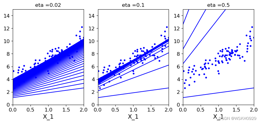
结论:从上图我们可以看出,当步长较小时,需要迭代较多次才可以收敛。当步长较大时,会导致在最优解附近来回摆动的情况出现。
4.2 随机梯度下降
theta_path_sgd = []
m = len(X_b)
n_epochs = 50
t0 = 5
t1 = 50


# 学习率衰减函数
def learning_schedule(t):
    return t0 / (t1 + t)


# 初始值
theta = np.random.randn(2, 1)

# 开始随机梯度下降
for epoch in range(n_epochs):
    for i in range(m):
        if epoch == 0 and i < 20:
            y_predict = X_new_b.dot(theta)
            plt.plot(X_new, y_predict, 'r-')
        # 随机选取一个样本进行梯度计算
        random_index = np.random.randint(m)
        xi = X_b[random_index:random_index + 1]
        yi = y[random_index:random_index + 1]
        # 计算梯度
        gradients = 2 * xi.T.dot(xi.dot(theta) - yi)
        # 根据梯度和步长更新theta值
        theta = theta - eta * gradients
        theta_path_sgd.append(theta)
        # 更新步长
        eta = learning_schedule(epoch * m + i)

# 画图
plt.plot(X, y, 'b.')
plt.axis([0, 2, 0, 15])
plt.show()

4.3 MiniBatch小批量随机梯度下降
theta_path_mgd = []
n_epochs = 200
minibatch = 16
theta = np.random.randn(2, 1)
t = 0
for epoch in range(n_epochs):
    shuffled_indices = np.random.permutation(m)
    X_b_shuffled = X_b[shuffled_indices]
    y_shuffled = y[shuffled_indices]
    for i in range(0, m, minibatch):
        t += 1
        xi = X_b_shuffled[i:i + minibatch]
        yi = y_shuffled[i:i + minibatch]
        gradients = 2 / minibatch * xi.T.dot(xi.dot(theta) - yi)
        eta = learning_schedule(t)
        theta = theta - eta * gradients
        theta_path_mgd.append(theta)

print(theta)
输出:
[[3.96882408]
 [3.03249021]]
4.4 不同梯度下降策略对比
theta_path_bgd = np.array(theta_path_bgd)
theta_path_sgd = np.array(theta_path_sgd)
theta_path_mgd = np.array(theta_path_mgd)

plt.figure(figsize=(8, 4))
plt.plot(theta_path_sgd[:, 0],
         theta_path_sgd[:, 1],
         'r-s',
         linewidth=1,
         label='SGD')
plt.plot(theta_path_mgd[:, 0],
         theta_path_mgd[:, 1],
         'g-+',
         linewidth=2,
         label='MINIGD')
plt.plot(theta_path_bgd[:, 0],
         theta_path_bgd[:, 1],
         'b-o',
         linewidth=3,
         label='BGD')
plt.axis([3,4,2.5,4.0])
plt.legend(loc='upper left')
plt.show()
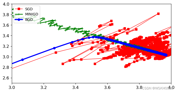
结论:
- BGD全批量梯度下降是比较平稳地在接近最优解,但比较耗时
- SGD随机梯度下降就比较混乱地接近最优解,但最不耗时
- MINIGD小批量随机梯度下降介于SGD和BGD中间,有一定随机性,但相对SGD更加平稳,且比BGD更快速
五、多项式回归
5.1 构造复杂数据集
m = 100
X = 6 * np.random.rand(m, 1) - 3
y = 0.5 * X**2 + X + np.random.randn(m, 1)
plt.scatter(X, y)

5.2 多项式特征提取+线性回归求解
from sklearn.preprocessing import PolynomialFeatures
from sklearn.linear_model import LinearRegression

# 多项式特征提取
poly_features = PolynomialFeatures(degree=2, include_bias=False)
# 提取特征
X_poly = poly_features.fit_transform(X)

# 定义线性回归器
lin_reg = LinearRegression()
# 用多项式提取器提取的特征进行训练
lin_reg.fit(X_poly, y)
# 系数
print(lin_reg.coef_)
# 截距
print(lin_reg.intercept_)
输出:
[[0.99343383 0.42940238]]
[0.18650351]
结论:输出 [0.99343383 0.42940238] 和 [0.18650351] 代表其拟合出来的方程为 0.18650351 + 0.99343383 X + 0.42940238 X 2 0.18650351+0.99343383X+0.42940238X^2 0.18650351+0.99343383X+0.42940238X2
和之前我们构造数据时设置的方程很接近:
0.5 X 2 + X + 随机扰动 0.5X^2+X+随机扰动 0.5X2+X+随机扰动
5.3 拟合曲线可视化
X_new = np.linspace(-3, 3, 100).reshape(100, 1)
X_new_poly = poly_features.transform(X_new)
y_new = lin_reg.predict(X_new_poly)
plt.plot(X, y, 'b.')
plt.plot(X_new, y_new, 'r-', label='prediction')
plt.axis([-3, 3, -5, 10])
plt.legend()
plt.show()

5.4 不同多项式拟合效果对比
from sklearn.pipeline import Pipeline
from sklearn.preprocessing import StandardScaler
for style, width, degree in (('g-', 2, 32), ('y-.', 4, 2), ('r-+', 3, 1)):
    poly_features = PolynomialFeatures(degree=degree, include_bias=False)
    std = StandardScaler()
    lin_reg = LinearRegression()
    polynomial_reg = Pipeline([('poly_features', poly_features),
                              ('StandardScaler', std), ('lin_reg', lin_reg)])
    polynomial_reg.fit(X, y)
    y_new_2 = polynomial_reg.predict(X_new)
    plt.plot(X_new, y_new_2, style, label="$degree=$"+str(degree), linewidth=width)
plt.plot(X, y, 'b.')
plt.axis([-3, 3, -5, 10])
plt.legend()
plt.show()

结论:degree太大容易过拟合
六、样本数量对结果的影响
from sklearn.metrics import mean_squared_error
from sklearn.model_selection import train_test_split
def plot_learning_curves(model,X,y):
    X_train,X_val,y_train,y_val, = train_test_split(X,y,test_size =0.2,random_state=0)
    train_errors,val_errors =[],[]
    for m in range(1,len(X_train)):
        model.fit(X_train[:m],y_train[:m])
        y_train_predict= model.predict(X_train[:m])
        y_val_predict =model.predict(X_val)
        train_errors.append(mean_squared_error(y_train[:m],y_train_predict[:m]))
        val_errors.append(mean_squared_error(y_val,y_val_predict))
    plt.xlabel("Train Size")
    plt.ylabel("MSE")
    plt.plot(np.sqrt(train_errors),'r-+',linewidth =2,label ='train_error')
    plt.plot(np.sqrt(val_errors),'b-',linewidth =3,label ='val_error')
    plt.legend()

lin_reg =LinearRegression()
plot_learning_curves(lin_reg,X,y)
plt.axis([0,80,0,3])
plt.show()

结论:样本量越大,训练集损失越大,测试集损失越小。样本量越小,测试集损失越小,训练集损失越大。
七、正则化
7.1 观察过拟合的现象
polynomial_reg = Pipeline([('poly_features',
                            PolynomialFeatures(degree=25, include_bias=False)),
                           ('lin_reg', LinearRegression())])
plot_learning_curves(polynomial_reg, X, y)
plt.axis([0, 80, 0, 5])
plt.show()

结论:可以看到degree很大时,模型过拟合的风险也很大
7.2 两种正则化
正则化的作用:缓解过拟合
7.2.1 岭回归正则化
岭回归正则化: J ( θ ) = MSE ( θ ) + α 1 2 ∑ i = 1 n θ i 2 岭回归正则化:J(\theta)=\operatorname{MSE}(\theta)+\alpha \frac{1}{2} \sum_{i=1}^n \theta_i^2 岭回归正则化:J(θ)=MSE(θ)+α21i=1∑nθi2
from sklearn.linear_model import Ridge

np.random.seed(42)
m = 20
X = 3 * np.random.rand(m, 1)
y = 0.5 * X + np.random.randn(m, 1) / 1.5 + 1
X_new = np.linspace(0, 3, 100).reshape(100, 1)


def plot_model(model_calss, polynomial, alphas, **model_kargs):
    for alpha, style in zip(alphas, ('b-', 'g--', 'r:')):
        model = model_calss(alpha, **model_kargs)
        if polynomial:
            model = Pipeline([('poly_features',
                               PolynomialFeatures(degree=10,
                                                  include_bias=False)),
                              ('StandardScaler', StandardScaler()),
                              ('lin_reg', model)])
        model.fit(X, y)
        y_new_regul = model.predict(X_new)
        lw = 2 if alpha > 0 else 1
        plt.plot(X_new,
                 y_new_regul,
                 style,
                 linewidth=lw,
                 label='alpha = {}'.format(alpha))
    plt.plot(X, y, 'b.', linewidth=3)
    plt.legend()


plt.figure(figsize=(14, 6))
plt.subplot(121)
plot_model(Ridge, polynomial=False, alphas=(0, 10, 100))
plt.subplot(122)
plot_model(Ridge, polynomial=True, alphas=(0, 10**-5, 1))
plt.show()
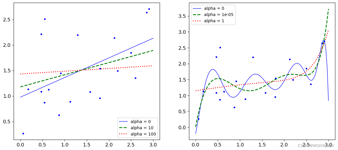
结论:参数alpha越大,惩罚力度越大,得到的结果越平稳,越不容易过拟合(但要考虑惩罚力度过大,会不会欠拟合)
7.2.2 Lasso回归正则化
L a s s o 回归正则化: J ( θ ) = MSE ( θ ) + α 1 2 ∑ i = 1 n ∣ θ i ∣ Lasso回归正则化:J(\theta)=\operatorname{MSE}(\theta)+\alpha \frac{1}{2} \sum_{i=1}^n |\theta_i| Lasso回归正则化:J(θ)=MSE(θ)+α21i=1∑n∣θi∣
from sklearn.linear_model import Lasso

plt.figure(figsize=(14, 6))
plt.subplot(121)
plot_model(Lasso, polynomial=False, alphas=(0, 0.1, 1))
plt.subplot(122)
plot_model(Lasso, polynomial=True, alphas=(0, 10**-1, 1))
plt.show()
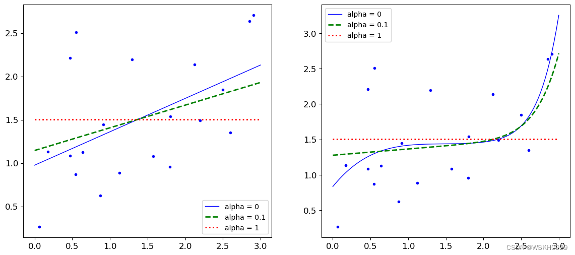
结论:和岭回归一致