吴恩达深度学习L1W4作业1
逐步构建你的深度神经网络
欢迎来到第4周作业的第1部分!在此之前你已经训练了一个2层的神经网络(只有一个隐藏层)。本周,你将学会构建一个任意层数的深度神经网络!
- 在此作业中,你将实现构建深度神经网络所需的所有函数。
- 在下一个作业中,你将使用这些函数来构建一个用于图像分类的深度神经网络。
完成此任务后,你将能够:
- 使用ReLU等非线性单位来改善模型
- 建立更深的神经网络(具有1个以上的隐藏层)
- 实现一个易于使用的神经网络类
符号说明:
- 上标
表示与
层相关的数量。
- 示例:是
层的激活。
和
是
- 上标
表示与
示例相关的数量。
- 示例:是第
- 下标
表示
- 示例:表示
让我们开始吧!
1 安装包
让我们首先导入作业过程中需要的所有包。
- numpy是Python科学计算的基本包。
- matplotlib是在Python中常用的绘制图形的库。
- dnn_utils为此笔记本提供了一些必要的函数。
- testCases提供了一些测试用例来评估函数的正确性
- np.random.seed(1)使所有随机函数调用保持一致。 这将有助于我们评估你的作业,请不要改变seed。
import numpy as np
import h5py
import matplotlib.pyplot as plt
from testCases_v2 import *
from dnn_utils_v2 import sigmoid, sigmoid_backward, relu, relu_backward%matplotlib inline
plt.rcParams['figure.figsize'] = (5.0, 4.0) # set default size of plots
plt.rcParams['image.interpolation'] = 'nearest'
plt.rcParams['image.cmap'] = 'gray'%load_ext autoreload
%autoreload 2np.random.seed(1)
2 作业大纲
为了构建你的神经网络,你将实现几个“辅助函数”。这些辅助函数将在下一个作业中使用,用来构建一个两层神经网络和一个L层的神经网络。你将实现的每个函数都有详细的说明,这些说明将指导你完成必要的步骤。此作业的大纲如下:
- 初始化两层的网络和
层的神经网络的参数。
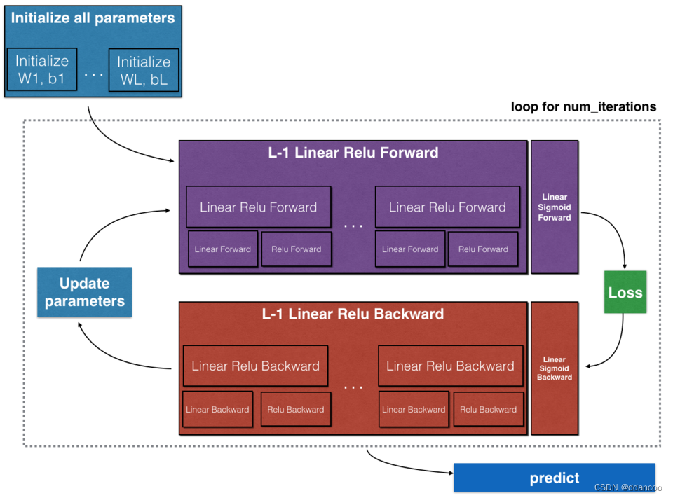
- 实现正向传播模块(在下图中以紫色显示)。
- 完成模型正向传播步骤的LINEAR部分()。
- 提供使用的ACTIVATION函数(relu / Sigmoid)。
- 将前两个步骤合并为新的[LINEAR-> ACTIVATION]前向函数。
- 堆叠[LINEAR-> RELU]正向函数L-1次(第1到L-1层),并在末尾添加[LINEAR-> SIGMOID](最后的 - 计算损失。
- 实现反向传播模块(在下图中以红色表示)。
- 完成模型反向传播步骤的LINEAR部分。
- 提供的ACTIVATE函数的梯度(relu_backward / sigmoid_backward)
- 将前两个步骤组合成新的[LINEAR-> ACTIVATION]反向函数。
- 将[LINEAR-> RELU]向后堆叠L-1次,并在新的L_model_backward函数中后向添加[LINEAR-> SIGMOID] - 最后更新参数。
注意:对于每个正向函数,都有一个对应的反向函数。 这也是为什么在正向传播模块的每一步都将一些值存储在缓存中的原因。缓存的值可用于计算梯度。 然后,在反向传导模块中,你将使用缓存的值来计算梯度。 此作业将指导说明如何执行这些步骤。
3 初始化
首先编写两个辅助函数用来初始化模型的参数。 第一个函数将用于初始化两层模型的参数。 第二个将把初始化过程推广到层模型上。
3.1 2层神经网络
说明:
- 模型的结构为:LINEAR -> RELU -> LINEAR -> SIGMOID。
- 随机初始化权重矩阵。 确保准确的维度,使用
np.random.randn(shape)* 0.01。 - 将偏差初始化为0。 使用
np.zeros(shape)。
# GRADED FUNCTION: initialize_parametersdef initialize_parameters(n_x, n_h, n_y):"""Argument:n_x -- size of the input layern_h -- size of the hidden layern_y -- size of the output layerReturns:parameters -- python dictionary containing your parameters:W1 -- weight matrix of shape (n_h, n_x)b1 -- bias vector of shape (n_h, 1)W2 -- weight matrix of shape (n_y, n_h)b2 -- bias vector of shape (n_y, 1)"""np.random.seed(1)### START CODE HERE ### (≈ 4 lines of code)W1=np.random.randn(n_h,n_x)b1=np.zeros((n_h,1))W2=np.random.randn(n_y,n_h)b2=np.zeros((n_y,1))### END CODE HERE ###assert(W1.shape == (n_h, n_x))assert(b1.shape == (n_h, 1))assert(W2.shape == (n_y, n_h))assert(b2.shape == (n_y, 1))parameters = {"W1": W1,"b1": b1,"W2": W2,"b2": b2}return parameters 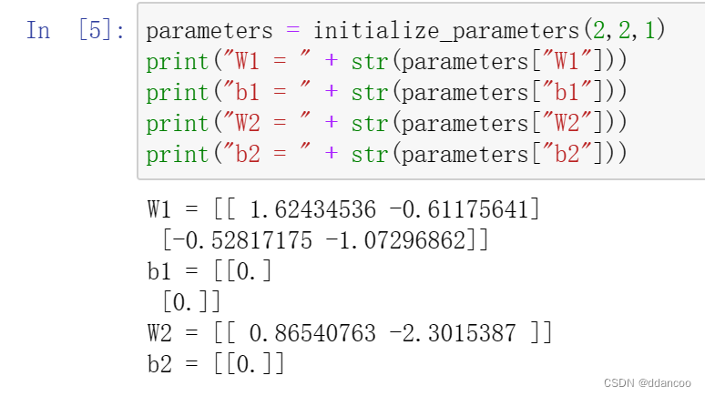
3.2 L层神经网络
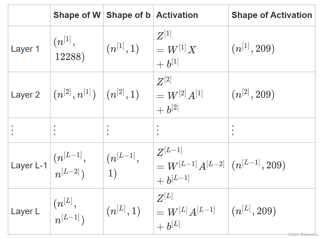
更深的L层神经网络的初始化更加复杂,因为存在更多的权重矩阵和偏差向量。 完成 initialize_parameters_deep后,应确保各层之间的维度匹配。 回想一下,是
层中的神经元数量。 因此,如果我们输入的 X 的大小为(12288,209)(以m=209为例),则:
当我们在python中计算W X +b时,使用广播,比如:


练习:实现L层神经网络的初始化。
说明:
- 模型的结构为 [LINEAR -> RELU] × (L-1) -> LINEAR -> SIGMOID。也就是说,L−1层使用ReLU作为激活函数,最后一层采用sigmoid激活函数输出。
- 随机初始化权重矩阵。使用
np.random.rand(shape)* 0.01。 - 零初始化偏差。使用
np.zeros(shape)。 - 我们将在不同的layer_dims变量中存储
,即不同层中的神经元数。例如,上周“二维数据分类模型”的
layer_dims为[2,4,1]:即有两个输入,一个隐藏层包含4个隐藏单元,一个输出层包含1个输出单元。因此,W1的维度为(4,2),b1的维度为(4,1),W2的维度为(1,4),而b2的维度为(1,1)。现在你将把它应用到L层! - 这是L=1 (一层神经网络)的实现。以启发你如何实现通用的神经网络(L层神经网络)。
if L == 1: parameters["W" + str(L)] = np.random.randn(layer_dims[1], layer_dims[0]) * 0.01 parameters["b" + str(L)] = np.zeros((layer_dims[1], 1))
# GRADED FUNCTION: initialize_parameters_deepdef initialize_parameters_deep(layer_dims):#eg:layer_dims为[5,4,3]代表了一共有3层,分别为输入层(5个神经元),隐藏层(4个神经元),输出层(3个神经元)。"""Arguments:layer_dims -- python array (list) containing the dimensions of each layer in our networkReturns:parameters -- python dictionary containing your parameters "W1", "b1", ..., "WL", "bL":Wl -- weight matrix of shape (layer_dims[l], layer_dims[l-1])bl -- bias vector of shape (layer_dims[l], 1)"""np.random.seed(3)parameters = {}L = len(layer_dims) # number of layers in the networkfor l in range(1, L):### START CODE HERE ### (≈ 2 lines of code)parameters['W'+str(l)]=np.random.randn(layer_dims[l],layer_dims[l-1])parameters['b'+str(l)]=np.zeros((layer_dims[l],1))### END CODE HERE ###assert(parameters['W' + str(l)].shape == (layer_dims[l], layer_dims[l-1]))assert(parameters['b' + str(l)].shape == (layer_dims[l], 1))return parameters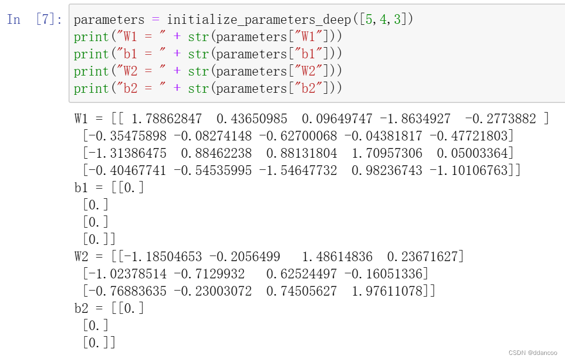
W1.shape=(layer_dims[1],layer_dims[0])=(4,5)
W2.shape=(layer_dims[2],layer_dims[1])=(3,4)
4 正向传播模块
4.1 线性正向
现在,你已经初始化了参数,接下来将执行正向传播模块。 首先实现一些基本函数,用于稍后的模型实现。按以下顺序完成三个函数:
- LINEAR
- LINEAR -> ACTIVATION,其中激活函数采用ReLU或Sigmoid。
- [LINEAR -> RELU] × (L-1) -> LINEAR -> SIGMOID(整个模型)
线性正向模块(在所有数据中均进行向量化)的计算按照以下公式:
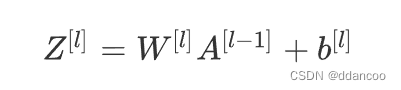
其中![]()
练习:建立正向传播的线性部分。
提醒:
该单元的数学表示为 ,你可能会发现
np.dot()有用。 如果维度不匹配,则可以printW.shape查看修改。
# GRADED FUNCTION: linear_forwarddef linear_forward(A, W, b):"""Implement the linear part of a layer's forward propagation.Arguments:A -- activations from previous layer (or input data): (size of previous layer, number of examples)W -- weights matrix: numpy array of shape (size of current layer, size of previous layer)b -- bias vector, numpy array of shape (size of the current layer, 1)Returns:Z -- the input of the activation function, also called pre-activation parameter cache -- a python dictionary containing "A", "W" and "b" ; stored for computing the backward pass efficiently"""### START CODE HERE ### (≈ 1 line of code)Z=np.dot(W,A)+b### END CODE HERE ###assert(Z.shape == (W.shape[0], A.shape[1]))#Z的维数(n^[l],m),W的维度(n^[l],n^[l-1]),l-1层的A的维度(n^[l-1],m)cache = (A, W, b)return Z, cache 
4.2 正向线性激活
在此笔记本中,你将使用两个激活函数:
Sigmoid:
![]()
我们为你提供了“ Sigmoid”函数。 该函数返回两项值:激活值"a"和包含"Z"的"cache"(这是我们将馈入到相应的反向函数的内容)。 你可以按下述方式得到两项值:
A, activation_cache = sigmoid(Z)
ReLU:
![]()
我们为你提供了relu函数。 该函数返回两项值:激活值“A”和包含“Z”的“cache”(这是我们将馈入到相应的反向函数的内容)。 你可以按下述方式得到两项值:
A, activation_cache = relu(Z)
为了更加方便,我们把两个函数(线性和激活)组合为一个函数(LINEAR-> ACTIVATION)。 因此,我们将实现一个函数用以执行LINEAR正向步骤和ACTIVATION正向步骤。
练习:实现 LINEAR->ACTIVATION 层的正向传播。 数学表达式为:![]()
其中激活"g" 可以是sigmoid()或relu()。 使用linear_forward()和正确的激活函数。
# GRADED FUNCTION: linear_activation_forwarddef linear_activation_forward(A_prev, W, b, activation):"""Implement the forward propagation for the LINEAR->ACTIVATION layerArguments:A_prev -- activations from previous layer (or input data): (size of previous layer, number of examples)W -- weights matrix: numpy array of shape (size of current layer, size of previous layer)b -- bias vector, numpy array of shape (size of the current layer, 1)activation -- the activation to be used in this layer, stored as a text string: "sigmoid" or "relu"Returns:A -- the output of the activation function, also called the post-activation value cache -- a python dictionary containing "linear_cache" and "activation_cache";stored for computing the backward pass efficiently"""if activation == "sigmoid":# Inputs: "A_prev, W, b". Outputs: "A, activation_cache".### START CODE HERE ### (≈ 2 lines of code)Z,linear_cache=linear_forward(A_prev,W,b)A,activation_cache=sigmoid(Z)### END CODE HERE ###elif activation == "relu":# Inputs: "A_prev, W, b". Outputs: "A, activation_cache".### START CODE HERE ### (≈ 2 lines of code)Z,linear_cache=linear_forward(A_prev,W,b)A,activation_cache=relu(Z)### END CODE HERE ###assert (A.shape == (W.shape[0], A_prev.shape[1]))cache = (linear_cache, activation_cache)return A, cache 
注意:在深度学习中,"[LINEAR->ACTIVATION]"计算被视为神经网络中的单个层,而不是两个层。
4.3 L层模型
为了方便实现层神经网络,你将需要一个函数来复制前一个函数(使用RELU的
linear_activation_forward)次,以及复制带有SIGMOID
linear_activation_forward。

图2 : [LINEAR -> RELU] × (L-1) -> LINEAR -> SIGMOID 模型
练习:实现上述模型的正向传播。
说明:在下面的代码中,变量AL表示
![]() 有时也称为
有时也称为Yhat,即。)
提示:
- 使用你先前编写的函数
- 使用for循环复制[LINEAR-> RELU](L-1)次
- 不要忘记在“cache”列表中更新缓存。 要将新值
c添加到list中,可以使用list.append(c)。 -
# GRADED FUNCTION: L_model_forwarddef L_model_forward(X, parameters):"""Implement forward propagation for the [LINEAR->RELU]*(L-1)->LINEAR->SIGMOID computationArguments:X -- data, numpy array of shape (input size, number of examples)parameters -- output of initialize_parameters_deep()Returns:AL -- last post-activation valuecaches -- list of caches containing:every cache of linear_relu_forward() (there are L-1 of them, indexed from 0 to L-2)the cache of linear_sigmoid_forward() (there is one, indexed L-1)"""caches = []A = X#A[0]=XL = len(parameters) // 2 # number of layers in the neural network# Implement [LINEAR -> RELU]*(L-1). Add "cache" to the "caches" list.for l in range(1, L):#l从1循环到l-1,使用RELU 激活函数来处理每一层的输出A_prev = A #先给上一层的A赋值### START CODE HERE ### (≈ 2 lines of code)A,cache=linear_activation_forward(A_prev,parameters['W'+str(l)],parameters['b'+str(l)],activation="relu")caches.append(cache)### END CODE HERE #### Implement LINEAR -> SIGMOID. Add "cache" to the "caches" list.### START CODE HERE ### (≈ 2 lines of code)AL,cache=linear_activation_forward(A,parameters['W'+str(L)],parameters['b'+str(L)],activation="sigmoid")caches.append(cache)#得到AL,对最后一层单独使用sigmoid激活函数### END CODE HERE ###assert(AL.shape == (1,X.shape[1]))return AL, caches
现在,你有了一个完整的正向传播模块,它接受输入X并输出包含预测的行向量。 它还将所有中间值记录在"caches"中以计算预测的损失值。
5 损失函数
现在,你将实现模型的正向和反向传播。 你需要计算损失,以检查模型是否在学习。
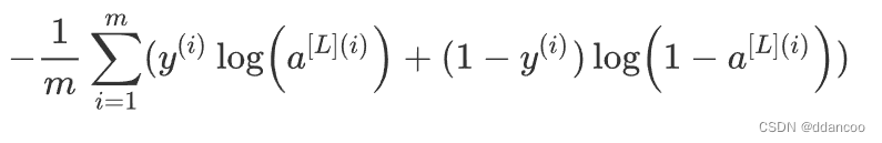
练习:使用以下公式计算交叉熵损失J:
# GRADED FUNCTION: compute_costdef compute_cost(AL, Y):"""Implement the cost function defined by equation (7).Arguments:AL -- probability vector corresponding to your label predictions, shape (1, number of examples)Y -- true "label" vector (for example: containing 0 if non-cat, 1 if cat), shape (1, number of examples)Returns:cost -- cross-entropy cost"""m = Y.shape[1]# Compute loss from aL and y.### START CODE HERE ### (≈ 1 lines of code)cost=-1/m*np.sum(Y*np.log(AL)+(1-Y)*np.log(1-AL),axis=1,keepdims=True)### END CODE HERE ###cost = np.squeeze(cost) # To make sure your cost's shape is what we expect (e.g. this turns [[17]] into 17).assert(cost.shape == ())return cost 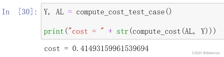
6 反向传播模块
就像正向传播一样,你将实现辅助函数以进行反向传播。 请记住,反向传播用于计算损失函数相对于参数的梯度。
提醒:

图3:
LINEAR->RELU->LINEAR->SIGMOID 的正向和反向传播,紫色块代表正向传播,红色块代表反向传播。
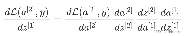
对于那些精通微积分的人(不必进行此作业),可以使用微积分的链式规则来得出2层网络中的损失 L相对于 的导数,如下所示:
为了计算梯度![]() ,请使用上一个链规则,然后执行
,请使用上一个链规则,然后执行![]() 。 在反向传播的每个步骤中,你都将当前梯度乘以对应层的梯度,以获得所需的梯度。
。 在反向传播的每个步骤中,你都将当前梯度乘以对应层的梯度,以获得所需的梯度。
同样地,为了计算梯度![]() ,你使用前一个链规则,然后执行
,你使用前一个链规则,然后执行![]() 。
。
这也是为什么我们称之为反向传播。
现在,类似于正向传播,你将分三个步骤构建反向传播:
- LINEAR backward
- LINEAR -> ACTIVATION backward,其中激活函数使用ReLU或sigmoid 的导数计算
- [LINEAR -> RELU] × (L-1) -> LINEAR -> SIGMOID backward(整个模型)
6.1 线性反向
对于层,线性部分为:![]() (之后是激活)。
(之后是激活)。
假设你已经计算出导数![]() 。你想获得
。你想获得![]()

图4
使用输入![]() 计算三个输出
计算三个输出![]() 。以下是所需的公式:
。以下是所需的公式:

练习:使用上面的3个公式实现linear_backward()。
# GRADED FUNCTION: linear_backwarddef linear_backward(dZ, cache):"""Implement the linear portion of backward propagation for a single layer (layer l)Arguments:dZ -- Gradient of the cost with respect to the linear output (of current layer l)cache -- tuple of values (A_prev, W, b) coming from the forward propagation in the current layerReturns:dA_prev -- Gradient of the cost with respect to the activation (of the previous layer l-1), same shape as A_prevdW -- Gradient of the cost with respect to W (current layer l), same shape as Wdb -- Gradient of the cost with respect to b (current layer l), same shape as b"""A_prev, W, b = cachem = A_prev.shape[1]### START CODE HERE ### (≈ 3 lines of code)dW=1/m*np.dot(dZ,A_prev.T)db=1/m*np.sum(dZ,axis=1,keepdims=True)dA_prev=np.dot(W.T,dZ)### END CODE HERE ###assert (dA_prev.shape == A_prev.shape)assert (dW.shape == W.shape)assert (db.shape == b.shape)return dA_prev, dW, db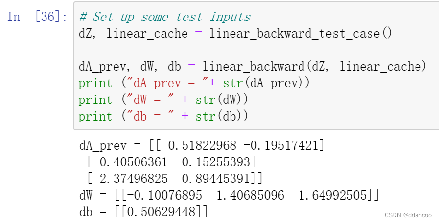
6.2 反向激活函数
接下来,创建一个合并两个辅助函数的函数:linear_backward 和反向步骤的激活 linear_activation_backward。
为了帮助你实现linear_activation_backward,我们提供了两个反向函数:
sigmoid_backward:实现SIGMOID单元的反向传播。 你可以这样使用:
dZ = sigmoid_backward(dA, activation_cache)
relu_backward:实现RELU单元的反向传播。 你可以这样使用:
dZ = relu_backward(dA, activation_cache)
如果g(.)是激活函数,sigmoid_backward和relu_backward计算
![]()
# GRADED FUNCTION: linear_activation_backwarddef linear_activation_backward(dA, cache, activation):"""Implement the backward propagation for the LINEAR->ACTIVATION layer.Arguments:dA -- post-activation gradient for current layer l cache -- tuple of values (linear_cache, activation_cache) we store for computing backward propagation efficientlyactivation -- the activation to be used in this layer, stored as a text string: "sigmoid" or "relu"Returns:dA_prev -- Gradient of the cost with respect to the activation (of the previous layer l-1), same shape as A_prevdW -- Gradient of the cost with respect to W (current layer l), same shape as Wdb -- Gradient of the cost with respect to b (current layer l), same shape as b"""linear_cache, activation_cache = cacheif activation == "relu":### START CODE HERE ### (≈ 2 lines of code)dZ=sigmoid_backward(dA,activation_cache)dA_prev,dW,db=linear_backward(dZ,linear_cache)#有了dZ才能算dA_prev,dW,db### END CODE HERE ###elif activation == "sigmoid":### START CODE HERE ### (≈ 2 lines of code)dZ=relu_backward(dA,activation_cache)dA_prev,dW,db=linear_backward(dZ,linear_cache)### END CODE HERE ###return dA_prev, dW, dbAL, linear_activation_cache = linear_activation_backward_test_case()dA_prev, dW, db = linear_activation_backward(AL, linear_activation_cache, activation = "sigmoid")
print ("sigmoid:")
print ("dA_prev = "+ str(dA_prev))
print ("dW = " + str(dW))
print ("db = " + str(db) + "\n")dA_prev, dW, db = linear_activation_backward(AL, linear_activation_cache, activation = "relu")
print ("relu:")
print ("dA_prev = "+ str(dA_prev))
print ("dW = " + str(dW))
print ("db = " + str(db))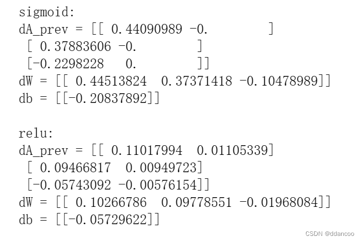
6.3 反向L层模型
现在,你将为整个网络实现反向传播函数。 回想一下,当你实现L_model_forward函数时,在每次迭代中,你都存储了一个包含(X,W,b和z)的缓存。 在反向传播模块中,你将使用这些变量来计算梯度。 因此,在L_model_backward函数中,你将从L层开始向后遍历所有隐藏层。在每个步骤中,你都将使用l层的缓存值反向传播到层l。 图5展示了反向传播过程。
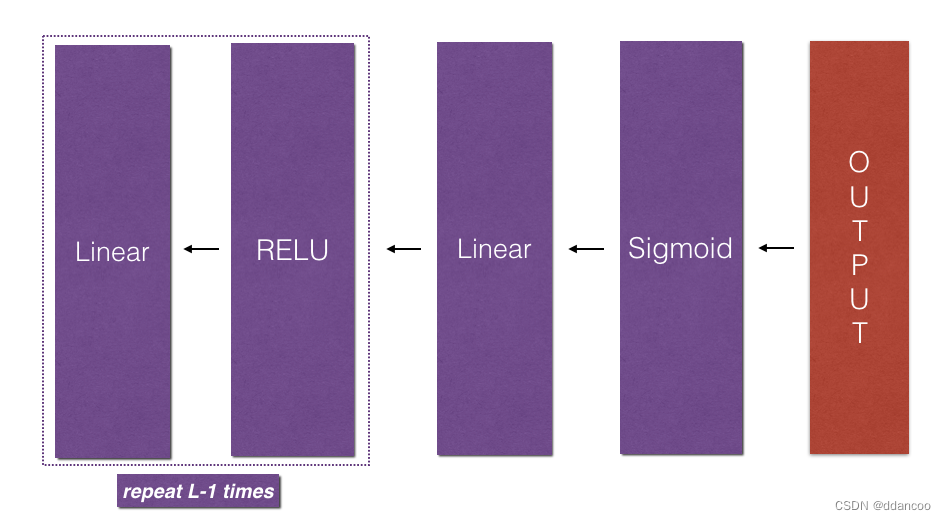
图5:反向流程
初始化反向传播:
为了使网络反向传播,我们知道输出是![]() 。因此,你的代码需要计算
。因此,你的代码需要计算dAL =![]() 。
。
为此,请使用以下公式(不需要深入的微积分知识):
dAL = - (np.divide(Y, AL) - np.divide(1 - Y, 1 - AL)) # derivative of cost with respect to AL
然后,你可以使用此激活后的梯度dAL继续反向传播。如图5所示,你现在可以将dAL输入到你实现的LINEAR-> SIGMOID反向函数中(它将使用L_model_forward函数存储的缓存值)。之后,你得通过for循环,使用LINEAR-> RELU反向函数迭代所有其他层。同时将每个dA,dW和db存储在grads词典中。为此,请使用以下公式:
![]()
例如,当l=3时,它将在grads["dW3"]中存储 。
练习:实现 [LINEAR->RELU] × (L-1) -> LINEAR -> SIGMOID 模型的反向传播。
# GRADED FUNCTION: L_model_backwarddef L_model_backward(AL, Y, caches):"""Implement the backward propagation for the [LINEAR->RELU] * (L-1) -> LINEAR -> SIGMOID groupArguments:AL -- probability vector, output of the forward propagation (L_model_forward())Y -- true "label" vector (containing 0 if non-cat, 1 if cat)caches -- list of caches containing:every cache of linear_activation_forward() with "relu" (it's caches[l], for l in range(L-1) i.e l = 0...L-2)the cache of linear_activation_forward() with "sigmoid" (it's caches[L-1])Returns:grads -- A dictionary with the gradientsgrads["dA" + str(l)] = ...grads["dW" + str(l)] = ...grads["db" + str(l)] = ..."""grads = {}#存储梯度L = len(caches) # 神经网络的层数,包括输入层和输出层m = AL.shape[1]#训练样本的数量Y = Y.reshape(AL.shape) # 将Y调整成和AL相同的形状# Initializing the backpropagation### START CODE HERE ### (1 line of code)dAL=-(np.divide(Y,AL)-np.divide(1-Y,1-AL))#处理dAL### END CODE HERE #### Lth layer (SIGMOID -> LINEAR) gradients. Inputs: "AL, Y, caches". Outputs: "grads["dAL"], grads["dWL"], grads["dbL"]### START CODE HERE ### (approx. 2 lines)current_cache=caches[L-1]#正向传播的最后一次grads["dA"+str(L)],grads["dW"+str(L)],grads["db"+str(L)]=linear_activation_backward(dAL,current_cache,activation="sigmoid")#处理在使用最后一次sigmoid激活函数往前倒推一次的其他参数### END CODE HERE ###for l in reversed(range(L - 1)):#从L-2层开始循环# lth layer: (RELU -> LINEAR) gradients.# Inputs: "grads["dA" + str(l + 2)], caches". Outputs: "grads["dA" + str(l + 1)] , grads["dW" + str(l + 1)] , grads["db" + str(l + 1)] ### START CODE HERE ### (approx. 5 lines)current_cache=caches[l]#获取之前的前向传播时保存的缓存dA_prev_temp,dW_temp,db_temp=linear_activation_backward(grads["dA"+str(l+2)],current_cache,activation="relu")#A_prev是上一层的A值#grads["dA" + str(l+2)] 存储的就是下一层的激活值的梯度。grads["dA"+str(l+1)]=dA_prev_tempgrads["dW"+str(l+1)]=dW_tempgrads["db"+str(l+1)]=db_temp#存储当前层其他参数的激活值### END CODE HERE ###return grads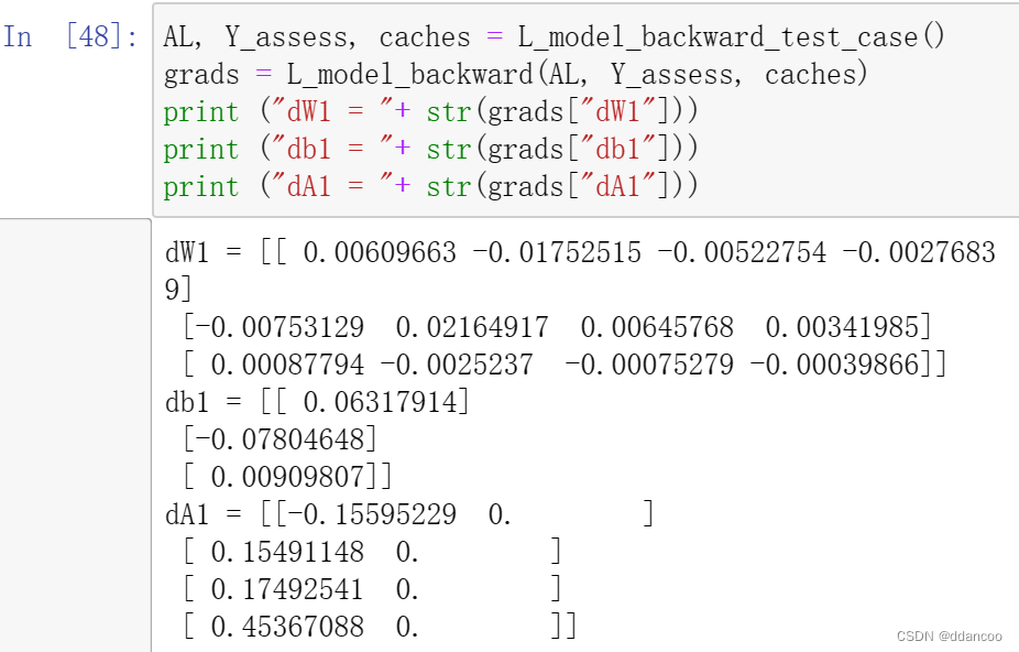
6.4 更新参数
在本节中,你将使用梯度下降来更新模型的参数:
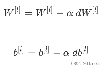
其中 α 是学习率。 在计算更新的参数后,将它们存储在参数字典中。
练习:实现update_parameters()以使用梯度下降来更新模型参数。
说明:
对于l=1,2,...,L,使用梯度下降更新每个 和
的参数。
# GRADED FUNCTION: update_parametersdef update_parameters(parameters, grads, learning_rate):"""Update parameters using gradient descentArguments:parameters -- python dictionary containing your parameters grads -- python dictionary containing your gradients, output of L_model_backwardReturns:parameters -- python dictionary containing your updated parameters parameters["W" + str(l)] = ... parameters["b" + str(l)] = ..."""L = len(parameters) // 2 # number of layers in the neural network# Update rule for each parameter. Use a for loop.### START CODE HERE ### (≈ 3 lines of code)for l in range(L):parameters["W"+str(l+1)]=parameters["W"+str(l+1)]-learning_rate*grads["dW"+str(l+1)]parameters["b"+str(l+1)]=parameters["b"+str(l+1)]-learning_rate*grads["db"+str(l+1)]#注意是反向传播,不要忘记是l+1 (ㄒoㄒ)### END CODE HERE ###return parameters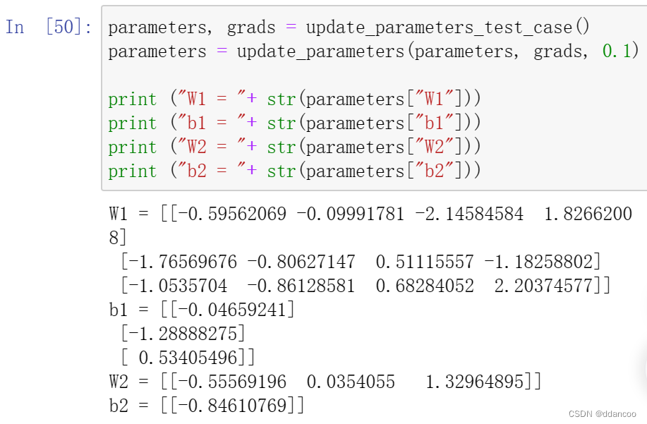
7 结论
恭喜你实现了构建深度神经网络所需的所有函数! (& 太艰难了(ㄒoㄒ))
我们知道这是一项艰巨的任务,但是继续前进将变得更好。 下一部分的作业相对容易。
在下一个作业中,你将使用这些函数构建两个模型用于分类猫图像和非猫图像:
- 两层神经网络
- L层神经网络