机器学习：多项式回归（Python）

多元线性回归闭式解：

closed_form_sol.py

import numpy as np
import matplotlib.pyplot as pltclass LRClosedFormSol:def __init__(self, fit_intercept=True, normalize=True):""":param fit_intercept: 是否训练bias:param normalize: 是否标准化数据"""self.theta = None  # 训练权重系数self.fit_intercept = fit_intercept  # 线性模型的常数项。也即偏置bias，模型中的theta0self.normalize = normalize  # 是否标准化数据if normalize:self.feature_mean, self.feature_std = None, None  # 特征的均值，标准方差self.mse = np.infty  # 训练样本的均方误差self.r2, self.r2_adj = 0.0, 0.0  # 判定系数和修正判定系数self.n_samples, self.n_features = 0, 0  # 样本量和特征数def fit(self, x_train, y_train):"""模型训练，根据是否标准化与是否拟合偏置项分类讨论:param x_train: 训练样本集:param y_train: 训练目标集:return:"""if self.normalize:self.feature_mean = np.mean(x_train, axis=0)  # 按样本属性计算样本均值self.feature_std = np.std(x_train, axis=0) + 1e-8  # 样本方差，为避免零除，添加噪声x_train = (x_train - self.feature_mean) / self.feature_std  # 标准化if self.fit_intercept:x_train = np.c_[x_train, np.ones_like(y_train)]  # 添加一列1，即偏置项样本# 训练模型self._fit_closed_form_solution(x_train, y_train)  # 求闭式解def _fit_closed_form_solution(self, x_train, y_train):"""线性回归的闭式解，单独函数，以便后期扩充维护:param x_train: 训练样本集:param y_train: 训练目标集:return:"""# pinv伪逆，即(A^T * A)^(-1) * A^Tself.theta = np.linalg.pinv(x_train).dot(y_train)  # 非正则化# xtx = np.dot(x_train.T, x_train) + 0.01 * np.eye(x_train.shape[1])  # 按公式书写# self.theta = np.dot(np.linalg.inv(xtx), x_train.T).dot(y_train)def get_params(self):"""返回线性模型训练的系数:return:"""if self.fit_intercept:  # 存在偏置项weight, bias = self.theta[:-1], self.theta[-1]else:weight, bias = self.theta, np.array([0])if self.normalize:  # 标准化后的系数weight = weight / self.feature_std.reshape(-1, 1)  # 还原模型系数bias = bias - weight.T.dot(self.feature_mean)return weight, biasdef predict(self, x_test):"""测试数据预测，x_test：待预测样本集，不包括偏置项1:param x_test::return:"""try:self.n_samples, self.n_features = x_test.shape[0], x_test.shape[1]except IndexError:self.n_samples, self.n_features = x_test.shape[0], 1  # 测试样本数和特征数if self.normalize:x_test = (x_test - self.feature_mean) / self.feature_std  # 测试数据标准化if self.fit_intercept:x_test = np.c_[x_test, np.ones(shape=x_test.shape[0])]  # 存在偏置项，添加一列1return x_test.dot(self.theta)def cal_mse_r2(self, y_pred, y_test):"""计算均方误差，计算拟合优度的判定系数R方和修正判定系数:param y_pred: 模型预测目标真值:param y_test: 测试目标真值:return:"""self.mse = ((y_test - y_pred) ** 2).mean()  # 均方误差# 计算测试样本的判定系数和修正判定系数self.r2 = 1 - ((y_test - y_pred) ** 2).sum() / ((y_test - y_test.mean()) ** 2).sum()self.r2_adj = 1 - (1 - self.r2) * (self.n_samples - 1) / (self.n_samples - self.n_features - 1)return self.mse, self.r2, self.r2_adjdef plt_predict(self, y_pred, y_test, is_show=True, is_sort=True):"""绘制预测值与真实值对比图:return:"""if self.mse is np.infty:self.cal_mse_r2(y_pred, y_test)if is_show:plt.figure(figsize=(7, 5))if is_sort:idx = np.argsort(y_test)plt.plot(y_pred[idx], "r:", lw=1.5, label="Predictive Val")plt.plot(y_test[idx], "k--", lw=1.5, label="Test True Val")else:plt.plot(y_pred, "r:", lw=1.5, label="Predictive Val")plt.plot(y_test, "k--", lw=1.5, label="Test True Val")plt.xlabel("Test sample observation serial number", fontdict={"fontsize": 12})plt.ylabel("Predicted sample value", fontdict={"fontsize": 12})plt.title("The predictive values of test samples \n MSE = %.5e, R2 = %.5f, R2_adj = %.5f"% (self.mse, self.r2, self.r2_adj), fontdict={"fontsize": 14})plt.legend(frameon=False)plt.grid(ls=":")if is_show:plt.show()

多项式构造

polynomial_feature.py

import numpy as npclass PolynomialFeatureData:"""生成特征多项式数据"""def __init__(self, x, degree, with_bias=False):"""参数初始化:param x: 采用数据，向量形式:param degree: 多项式最高阶次:param with_bias: 是否需要偏置项"""self.x = np.asarray(x)self.degree = degreeself.with_bias = with_biasif with_bias:self.data = np.zeros((len(x), degree + 1))else:self.data = np.zeros((len(x), degree))def fit_transform(self):"""构造多项式特征数据:return:"""if self.with_bias:self.data[:, 0] = np.ones(len(self.x))self.data[:, 1] = self.x.reshape(-1)for i in range(2, self.degree + 1):self.data[:, i] = (self.x ** i).reshape(-1)else:self.data[:, 0] = self.x.reshape(-1)for i in range(1, self.degree):self.data[:, i] = (self.x ** (i + 1)).reshape(-1)return self.dataif __name__ == '__main__':x = np.random.randn(5)feat_obj = PolynomialFeatureData(x, 5, with_bias=True)data = feat_obj.fit_transform()print(data)

 多项式回归

test_polynomial_fit.py

import numpy as np
import matplotlib.pyplot as plt
from polynomial_feature import PolynomialFeatureData
from closed_form_sol import LRClosedFormSoldef objective_fun(x):"""目标函数，假设一个随机二次多项式:param x: 采样数据，向量:return:"""return 0.5 * x ** 2 + x + 2np.random.seed(42)  # 随机种子，以便结果可再现
n = 30  # 样本量
raw_x = np.sort(6 * np.random.rand(n, 1) - 3)  # 采样数据[-3, 3]，均匀分布
raw_y = objective_fun(raw_x) + 0.5 * np.random.randn(n, 1)  # 目标值，添加噪声degree = [1, 2, 5, 10, 15, 20]  # 拟合多项式的最高阶次
plt.figure(figsize=(15, 8))
for i, d in enumerate(degree):feature_obj = PolynomialFeatureData(raw_x, d, with_bias=False)  # 特征数据对象X_samples = feature_obj.fit_transform()  # 生成特征多项式数据lr_cfs = LRClosedFormSol()  # 采用线性回归求解多项式回归lr_cfs.fit(X_samples, raw_y)  # 求解多项式回归系数theta = lr_cfs.get_params()  # 获得系数print("degree: %d, theta is " %d, theta[0].reshape(-1)[::-1], theta[1])y_train_pred = lr_cfs.predict(X_samples)  # 在训练集上的预测# 测试样本采样X_test_raw = np.linspace(-3, 3, 150)  # 测试数据y_test = objective_fun(X_test_raw)  # 测试数据的真值feature_obj = PolynomialFeatureData(X_test_raw, d, with_bias=False)  # 特征数据对象X_test = feature_obj.fit_transform()  # 生成特征多项式数据y_test_pred = lr_cfs.predict(X_test)  # 模型在测试样本上的预测值# 可视化不同阶次下的多项式拟合曲线plt.subplot(231 + i)plt.scatter(raw_x, raw_y, edgecolors="k", s=15, label="Raw Data")plt.plot(X_test_raw, y_test, "k-", lw=1, label="Objective Fun")plt.plot(X_test_raw, y_test_pred, "r--", lw=1.5, label="Polynomial Fit")plt.legend(frameon=False)plt.grid(ls=":")plt.xlabel("$x$", fontdict={"fontsize": 12})plt.ylabel("$y(x)$", fontdict={"fontsize": 12})test_ess = (y_test_pred.reshape(-1) - y_test) ** 2  # 误差平方test_mse, test_std = np.mean(test_ess), np.std(test_ess)train_ess = (y_train_pred - raw_y) ** 2  # 误差平方train_mse, train_std = np.mean(train_ess), np.std(train_ess)plt.title("Degree {} Test Mse = {:.2e}(+/-{:.2e}) \n Train Mse = {:.2e}(+/-{:.2e})".format(d, test_mse, test_std, train_mse, train_std))plt.axis([-3, 3, 0, 9])
plt.tight_layout()
plt.show()

输出结果：

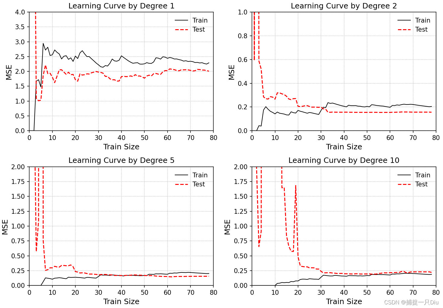
学习曲线

learning_curve1.py

import numpy as np
import matplotlib.pyplot as plt
from polynomial_feature import PolynomialFeatureData
from closed_form_sol import LRClosedFormSol
from sklearn.model_selection import train_test_splitdef objective_fun(x):"""目标函数，假设一个随机二次多项式:param x: 采样数据，向量:return:"""return 0.5 * x ** 2 + x + 2np.random.seed(42)  # 随机种子，以便结果可再现
n = 100  # 样本量
raw_x = np.sort(6 * np.random.rand(n, 1) - 3)  # 采样数据[-3, 3]，均匀分布
raw_y = objective_fun(raw_x) + 0.5 * np.random.randn(n, 1)  # 目标值，添加噪声degree = [1, 2, 5, 10]  # 拟合阶次
plt.figure(figsize=(10, 7))  # 图像尺寸
for i, d in enumerate(degree):# 生成特征多项式对象，包含偏置项feta_obj = PolynomialFeatureData(raw_x, d, with_bias=False)X_sample = feta_obj.fit_transform()  # 生成特征多项式数据X_train, X_test, y_train, y_test = \train_test_split(X_sample, raw_y, test_size=0.2, random_state=0)train_mse, test_mse = [], []  # 随样本量的增加，训练误差和测试误差for j in range(1, 80):lr_cfs = LRClosedFormSol()  # 线性回归闭式解theta = lr_cfs.fit(X_train[:j, :], y_train[:j])  # 拟合多项式y_test_pred = lr_cfs.predict(X_test)  # 测试样本预测y_train_pred = lr_cfs.predict(X_train[:j, :])  # 训练样本预测train_mse.append(np.mean((y_train_pred.reshape(-1) - y_train[:j].reshape(-1)) ** 2))test_mse.append(np.mean((y_test_pred.reshape(-1) - y_test.reshape(-1)) ** 2))# 可视化多项式拟合曲线plt.subplot(221 + i)plt.plot(train_mse, "k-", lw=1, label="Train")plt.plot(test_mse, "r--", lw=1.5, label="Test")plt.legend(frameon=False)plt.grid(ls=":")plt.xlabel("Train Size", fontdict={"fontsize": 12})plt.ylabel("MSE", fontdict={"fontsize": 12})plt.title("Learning Curve by Degree {}".format(d))if i == 0:plt.axis([0, 80, 0, 4])if i == 1:plt.axis([0, 80, 0, 1])if i in [2, 3]:plt.axis([0, 80, 0, 2])
plt.tight_layout()
plt.show()

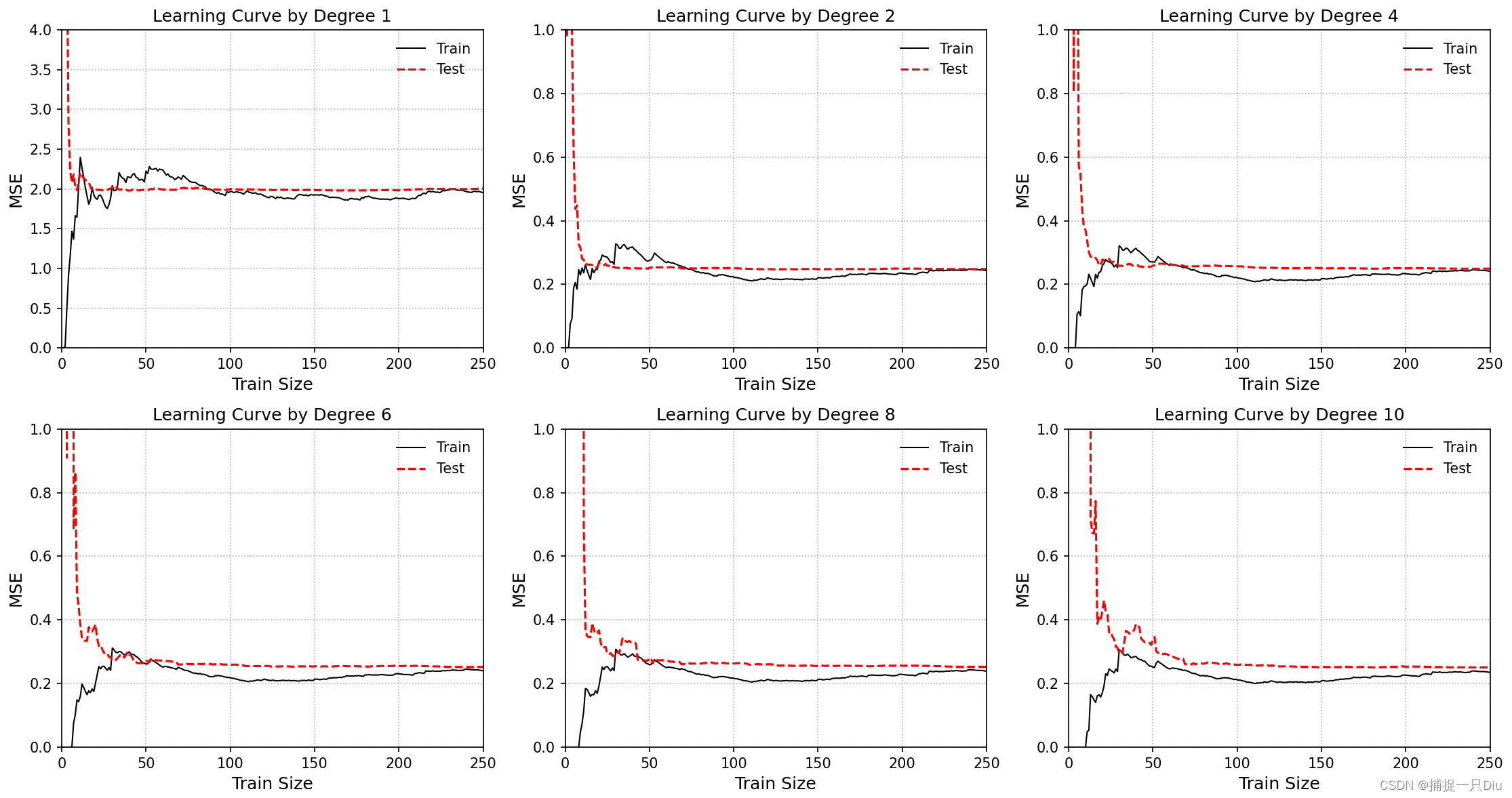
学习曲线（采用10折交叉验证）

learning_curve2.py

import numpy as np
import matplotlib.pyplot as plt
from polynomial_feature import PolynomialFeatureData
from closed_form_sol import LRClosedFormSol
from sklearn.model_selection import KFolddef objective_fun(x):"""目标函数，假设一个随机二次多项式:param x: 采样数据，向量:return:"""return 0.5 * x ** 2 + x + 2np.random.seed(42)  # 随机种子，以便结果可再现
n = 300  # 样本量
raw_x = np.sort(6 * np.random.rand(n, 1) - 3)  # 采样数据[-3, 3]，均匀分布
raw_y = objective_fun(raw_x) + 0.5 * np.random.randn(n, 1)  # 目标值，添加噪声k_fold = KFold(n_splits=10)  # 划分为10折
degree = [1, 2, 4, 6, 8, 10]  # 拟合阶次
plt.figure(figsize=(15, 8))  # 图像尺寸
for i, d in enumerate(degree):# 生成特征多项式对象，包含偏置项feta_obj = PolynomialFeatureData(raw_x, d, with_bias=False)X_sample = feta_obj.fit_transform()  # 生成特征多项式数据train_mse, test_mse = [], []  # 随样本量的增加，训练误差和测试误差for j in range(1, 270):train_mse_, test_mse_ = 0.0, 0.0  # 交叉验证for idx_train, idx_test in k_fold.split(raw_x, raw_y):X_train, y_train = X_sample[idx_train], raw_y[idx_train]X_test, y_test = X_sample[idx_test], raw_y[idx_test]lr_cfs = LRClosedFormSol()  # 线性回归闭式解theta = lr_cfs.fit(X_train[:j, :], y_train[:j])  # 拟合多项式y_test_pred = lr_cfs.predict(X_test)  # 测试样本预测y_train_pred = lr_cfs.predict(X_train[:j, :])  # 训练样本预测train_mse_ += np.mean((y_train_pred.reshape(-1) - y_train[:j].reshape(-1)) ** 2)test_mse_ += np.mean((y_test_pred.reshape(-1) - y_test.reshape(-1)) ** 2)train_mse.append(train_mse_ / 10)test_mse.append(test_mse_ / 10)# 可视化多项式拟合曲线plt.subplot(231 + i)plt.plot(train_mse, "k-", lw=1, label="Train")plt.plot(test_mse, "r--", lw=1.5, label="Test")plt.legend(frameon=False)plt.grid(ls=":")plt.xlabel("Train Size", fontdict={"fontsize": 12})plt.ylabel("MSE", fontdict={"fontsize": 12})plt.title("Learning Curve by Degree {}".format(d))if i == 0:plt.axis([0, 250, 0, 4])else:plt.axis([0, 250, 0, 1])
plt.tight_layout()
plt.show()