当前位置：首页 > news >正文

②单细胞学习-组间及样本细胞比例分析

news 来源：原创 2024/9/28 23:29:43

数据读入

每个样本各细胞比例

两个组间细胞比例

亚组间细胞比例差异分析（循环）

单个细胞类型亚新间比例差异

①单细胞学习-数据读取、降维和分群-CSDN博客

比较各个样本间的各类细胞比例或者亚组之间的细胞比例差异

①数据读入

#各样本细胞比例计算
rm(list = ls()) 
library(Seurat)
load("scedata1.RData")#这里是经过质控和降维后的单细胞数据
table(scedata$orig.ident)#查看各组细胞数
table(Idents(scedata))#查看各种类型细胞数目
#prop.table(table(Idents(scedata)))
table(Idents(scedata), scedata$orig.ident)#每个样本不同类型细胞数据

> table(scedata$orig.ident)#查看各组细胞数BM1  BM2  BM3  GM1  GM2  GM3 
2754  747 2158 1754 1528 1983

> table(Idents(scedata))#查看各种类型细胞数目Fibroblast Endothelial      Immune       Other  Epithelial 2475        4321        2688         766         674 
> #prop.table(table(Idents(scedata)))
> table(Idents(scedata), scedata$orig.ident)#每个样本不同类型细胞数据BM1  BM2  BM3  GM1  GM2  GM3Fibroblast   571  135  520  651  312  286Endothelial  752  244  619  716  906 1084Immune      1220  145  539  270  149  365Other        142  161  194   55   79  135Epithelial    69   62  286   62   82  113

②每个样本各细胞比例

#换算每样样本每种细胞占有的比例:绘制总的堆积图
Cellratio <- prop.table(table(Idents(scedata),scedata$orig.ident),margin = 2)# margin = 2按照列计算每个样本比例
Cellratio <- as.data.frame(Cellratio)#计算比例绘制堆积图
library(ggplot2)#绘制细胞比例堆积图
colourCount = length(unique(Cellratio$Var1))
p1 <- ggplot(Cellratio) + geom_bar(aes(x =Var2, y= Freq, fill = Var1),stat = "identity",width = 0.7,size = 0.5,colour = '#222222')+ theme_classic() +labs(x='Sample',y = 'Ratio')+#coord_flip()+ #进行翻转theme(panel.border = element_rect(fill=NA,color="black", size=0.5, linetype="solid"))
p1
dev.off()

> head(Cellratio)Var1 Var2       Freq
1  Fibroblast  BM1 0.20733479
2 Endothelial  BM1 0.27305737
3      Immune  BM1 0.44299201
4       Other  BM1 0.05156137
5  Epithelial  BM1 0.02505447
6  Fibroblast  BM2 0.18072289

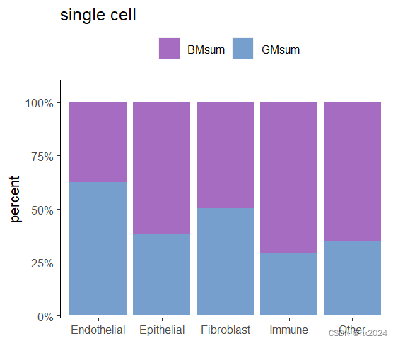
③两个组间细胞比例

这里比较BM和GM两个组间的细胞比例

##分成两个组进行比较:先查看每个样本的具体细胞数量
library(tidyverse)
library(reshape)
clusdata <- as.data.frame(table(Idents(scedata), scedata$orig.ident))
#进行长宽数据转换
clusdata1 <- clusdata %>% pivot_wider(names_from = Var2,values_from =Freq )
clusdata1 <- as.data.frame(clusdata1)
rownames(clusdata1) <- clusdata1$Var1
clusdata2 <- clusdata1[,-1]#[1] "BM1" "BM2" "BM3" "GM1" "GM2" "GM3"
#分别计算每个组每种细胞和
BM <- c("BM1","BM2","BM3")
clusdata2$BMsum <- rowSums(clusdata2[,BM])
GM <- c("GM1","GM2","GM3")
clusdata2$GMsum <- rowSums(clusdata2[,GM])#然后绘制堆积图
clus2 <- clusdata2[,c(7,8)]
clus2$ID <- rownames(clus2)
clus3  <- melt(clus2, id.vars = c("ID"))##根据分组变为长数据
p <- ggplot(data = clus3,aes(x=ID,y=value,fill=variable))+#geom_bar(stat = "identity",position = "stack")+    ##展示原来数值geom_bar(stat = "identity",position = "fill")+      ##按照比例展示:纵坐标为1scale_y_continuous(expand = expansion(mult=c(0.01,0.1)),##展示纵坐标百分比数值labels = scales::percent_format())+scale_fill_manual(values = c("BMsum"="#a56cc1","GMsum"="#769fcd"),       ##配色："BMsum"="#98d09d","GMsum"="#e77381"limits=c("BMsum","GMsum"))+                            ##limit调整图例顺序theme(panel.background = element_blank(),          ##主题设置axis.line = element_line(),                   legend.position = "top")+                  #"bottom"labs(title = "single cell",x=NULL,y="percent")+           ##X，Y轴设置guides(fill=guide_legend(title = NULL,nrow = 1,byrow = FALSE))
p
dev.off()

> head(clus3)ID variable value
1  Fibroblast    BMsum  1226
2 Endothelial    BMsum  1615
3      Immune    BMsum  1904
4       Other    BMsum   497
5  Epithelial    BMsum   417
6  Fibroblast    GMsum  1249

④亚组间细胞比例差异分析（循环）

#组间差异分析：仍然是使用这个比例数据进行分析，不过却是在各个样本中进行比例比较
table(scedata$orig.ident)#查看各组细胞数
table(Idents(scedata))#查看各种类型细胞数目
table(Idents(scedata), scedata$orig.ident)#各组不同细胞群细胞数
Cellratio <- prop.table(table(Idents(scedata), scedata$orig.ident), margin = 2)#计算各组样本不同细胞群比例
Cellratio <- data.frame(Cellratio)
#需要进行数据转换,计算每个样本比例后进行差异分析
library(reshape2)
cellper <- dcast(Cellratio,Var2~Var1, value.var = "Freq")
rownames(cellper) <- cellper[,1]
cellper <- cellper[,-1]
###添加分组信息dataframe
sample <- c("BM1","BM2","BM3","GM1","GM2","GM3")
group <- c("BM","BM","BM","GM","GM","GM")
samples <- data.frame(sample, group)#创建数据框
rownames(samples)=samples$sample
cellper$sample <- samples[rownames(cellper),'sample']#R添加列
cellper$group <- samples[rownames(cellper),'group']#R添加列###作图展示
pplist = list()##循环作图建立空表
library(ggplot2)
library(dplyr)
library(ggpubr)
library(cowplot)
sce_groups = c('Endothelial','Fibroblast','Immune','Epithelial','Other')
for(group_ in sce_groups){cellper_  = cellper %>% select(one_of(c('sample','group',group_)))#选择一组数据colnames(cellper_) = c('sample','group','percent')#对选择数据列命名cellper_$percent = as.numeric(cellper_$percent)#数值型数据cellper_ <- cellper_ %>% group_by(group) %>% mutate(upper =  quantile(percent, 0.75), lower = quantile(percent, 0.25),mean = mean(percent),median = median(percent))#上下分位数print(group_)print(cellper_$median)pp1 = ggplot(cellper_,aes(x=group,y=percent)) + #ggplot作图geom_jitter(shape = 21,aes(fill=group),width = 0.25) + stat_summary(fun=mean, geom="point", color="grey60") +#stat_summary添加平均值theme_cowplot() +theme(axis.text = element_text(size = 10),axis.title = element_text(size = 10),legend.text = element_text(size = 10),legend.title = element_text(size = 10),plot.title = element_text(size = 10,face = 'plain'),legend.position = 'none') + labs(title = group_,y='Percentage') +geom_errorbar(aes(ymin = lower, ymax = upper),col = "grey60",width =  1)###组间t检验分析labely = max(cellper_$percent)compare_means(percent ~ group,  data = cellper_)my_comparisons <- list( c("GM", "BM") )pp1 = pp1 + stat_compare_means(comparisons = my_comparisons,size = 3,method = "t.test")pplist[[group_]] = pp1
}#批量绘制
plot_grid(pplist[['Endothelial']],pplist[['Fibroblast']],pplist[['Immune']],pplist[['Epithelial']],pplist[['Other']],#nrow = 5,#列数ncol = 5)#行数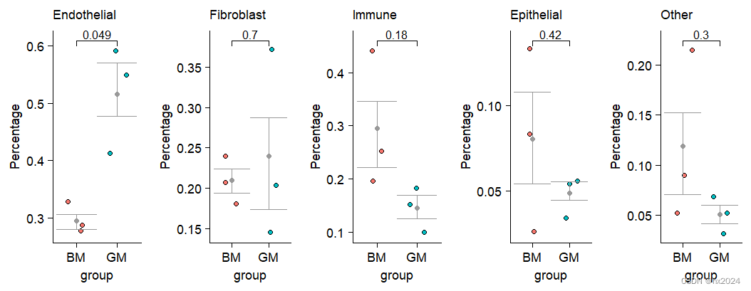

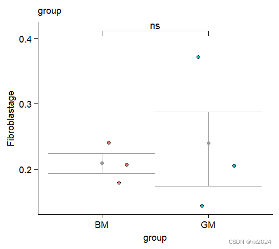
⑤单个细胞类型亚新间比例差异

##数据处理
##单个细胞类型比例计算
rm(list = ls()) 
library(Seurat)
library(tidyverse)
library(reshape2)
library(ggplot2)
library(dplyr)
library(ggpubr)
library(cowplot)
load("scedata1.RData")#计算各个样本细胞，各种类型细胞
Cellratio <- prop.table(table(Idents(scedata), scedata$orig.ident), margin = 2)#计算样本比例
Cellratio <- data.frame(Cellratio)
cellper <- dcast(Cellratio,Var2~Var1, value.var = "Freq")##长数据转宽数据
rownames(cellper) <- cellper[,1]
cellper <- cellper[,-1]
sample <- c("BM1","BM2","BM3","GM1","GM2","GM3")###添加分组信息dataframe
group <- c("BM","BM","BM","GM","GM","GM")
samples <- data.frame(sample, group)#创建数据框
rownames(samples)=samples$sample
cellper$sample <- samples[rownames(cellper),'sample']#R添加列
cellper$group <- samples[rownames(cellper),'group']#R添加列dat <- cellper[,c(1,7)]#提取需要分析的细胞类型"Fibroblast" "group"  
#根据分组计算四分位及中位数
dat1 <- dat %>% group_by(group) %>% mutate(upper =  quantile(Fibroblast, 0.75), lower = quantile(Fibroblast, 0.25),mean = mean(Fibroblast),median = median(Fibroblast))
#table(dat1$group)#BM GM

作图

#pdf("单个细胞类型组间比较.pdf",width = 4,height = 4)##一定添加大小
my_comparisons =list( c("BM","GM"))
P <- ggplot(dat1,aes(x=group,y= Fibroblast)) + #ggplot作图geom_jitter(shape = 21,aes(fill=group),width = 0.25) + stat_summary(fun=mean, geom="point", color="grey60") +theme_cowplot() +theme(axis.text = element_text(size = 10),axis.title = element_text(size = 10),legend.text = element_text(size = 10),legend.title = element_text(size = 10),plot.title = element_text(size = 10,face = 'plain'),legend.position = 'none') + labs(title = "group",y='Fibroblastage') +geom_errorbar(aes(ymin = lower, ymax = upper),col = "grey60",width =  1)+#误差棒#差异检验stat_compare_means(comparisons=my_comparisons,label.y = c(0.4),method="t.test",#wilcox.testlabel="p.signif")
P
dev.off()