Crafting 手工 Physically Motivated Shading Models for Game Development

http://renderwonk.com/publications/s2010-shading-course/hoffman/s2010_physically_based_shading_hoffman_b_notes.pdf

motivation and infrastructure 基础知识
motivation
the first question many game developers ask in connection with physically-based shading models is “why bother?”. this is a valid question, since games do not aim at an exact physical simulation of light transport. however, we shall see many practical advantages for games in adopting these methods.

with shading models that are based on physical principles, it is easier to achieve photorealistic and cinematic looks. objects that use such shading models retain their basic appearance when the lighting and viewing conditions change; they have a roubustness that is often not afforded by ad-hoc shading hacks. art asset creation is also easier; less “slider tweaking” and adjustment of “fudge factors” is needed to achieve high visual quality, and the material interface exposed to the artists is simple, powerful and expressive.

for graphics programmers and shader writers, physically based shaders are easier to troubleshoot. when sth. appears to bright, too dark, too green, too thiny, etc. then it is much easier to reason about what is happening in the shader when the various terms and parameters have a physical meaning. it is also easier to extend such shaders to add new features, since physical reasoning can be userd to determine e.g, which which subexpression in the shader should be affected by ambient occlusion, or how an environment map should be combined with existing shading terms.
there have been several articles in the press over the last few years [28,29,30] highlighting these advantages in the case of film production; most of the content of these articles applies equally to game development.

infrastructure
there are several basic features a game rendering engine needs to have to get the most benefit from physicall-based shading models. shading needs to occur in linear space, with inputs and outputs correctly transformed (gamma-correct rendering), the engine should have some support for lighting and shading values with high dynamic range (HDR), and there needs to be an appropriate transformation from scene to display colors (tone mapping).

gamma-correct rendering
when artists author shader inputs such as textures, light colors, and vertex colors, a non-linear encoding is typically used for numerical representation and storage. this means that physical light intensities are not linearly proportional to numerical values. pixel values stored in the frame buffer after rendering use similar nonlinear encodings.

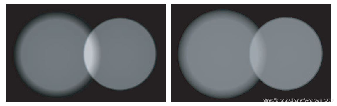
firgure 1: this firgure shows a grey flat surface illuminated by two overlapping spotlights. in the left image, shading computations have been performed on nonlinear (sRGB) encoded values, so the addtion of the two lights in the overlapping region results in an overly bright region that does not correspond to the expected brightness from summing the two lights. on the right the shading computations are performed on linearly encoded values, and the result appears correct. (image from “real-time rendering, 3rd edition”, used with permission from A K Peters)

these encodings are primarily used to make efficient use of limited bit precision. although such nonlinear encodings have steps between successive integers values which are not physically uniform (the amount of light energy added at each step varies over the range), they are (somewhat) perceptually uniform (the perceived change in brightness at each step does not vary much over the range). this allows for fewer bits to be used without banding.
the two nonlinear encodings most commonly used in game graphics are sRGB (used by computer monitors) and ITU-R recommendation BT.709 (used by HDTV displays). The o±cial sRGB spec-
i¯cation is the IEC 61966-2-1:1999 standard, a working draft of which is available online [18]. Both
standards are described in detail elsewhere on the Internet, and in a comprehensive book on video
encoding by Charles Poynton [26].

since shading inputs and outputs use nonlinear encodings, then by default shading computations will be performed on nonlinearly encoded values, which is incorrect and can lead to “1+1=3” situations such as the one shown in figure 1. to avoid this, shading inputs need to be converted to linear values, and the shader output needs to be converted to the appropriate nonlinear encoding. in principle, these conversions can be done in hardware by the GPU (for textures and render targets) or in a post-process (for shader constants and vertex colors).

although converting a game engine to linear shading generally improves visuals, there are often unintented consequences that need to be addressed. light distance falloff, Lambert falloff, spotlight angular falloff, soft shadow edge feathering, vertex interpolation all will appear differently now that they are happening in linear space. this may require some retraining or readjustment by the artists, and a few rare cases (like vertex interpolation) might need to be fixed in the shader.

more details on how to convert a game engine to be gamma-correct can be found online[10,16,35].

making an ad-hoc game shading model physically plausible
the initial generations of graphics accelerators did not have programmable shaders, and impose a fixed-function shading model on games for several years. once programmble shading was introduced, game developers were used to the fixed-funtion models and often extend them instead of developing new models from scratch. for this reason, many physically incorrect properties of the old fixed-function model persist in common usage today.

we will start with a fairly representative game shading model based on phong’s original model[25]. we will show here the equation for a single punctual light source (note that a game will typically have multiple punctual lights and additional terms for ambient light, environment maps, etc.):

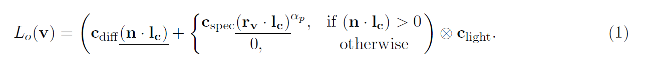
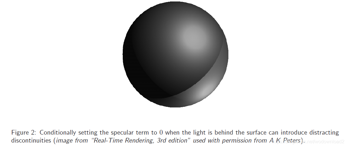
like the clamp on the diffuse dot product, the conditional on the specular term is there to remove the conditions of punctual lights behind the surface. howver, this condition does not make physical sense and worse, can introduce severe artifacts (see figure 2).

we will modify the shader to avoid specular from backfacing lights in a different way. instead of a conditional, we will multiply the specular term by
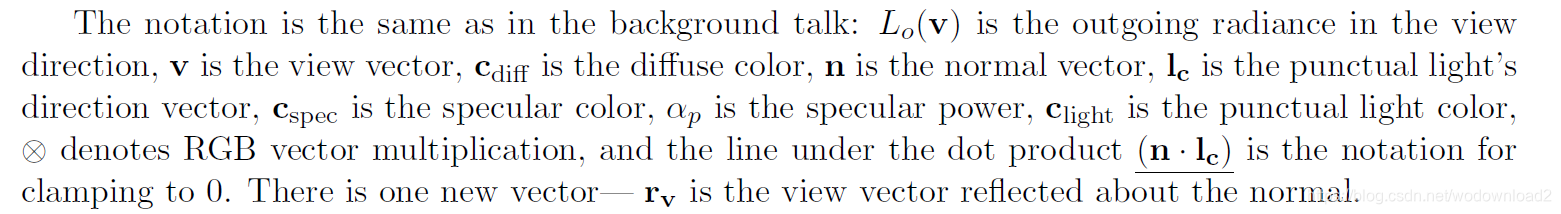
this makes sense since this cosine term is not actually part of the BRDF, but of the rendering equation. recall the punctual light rendering equation from the background talk in this course:

after replacing the conditional with multiplication by the cosine term, we get the following equation, which is simpler, faster to compute, and does not suffer from discontinuity artifacts:

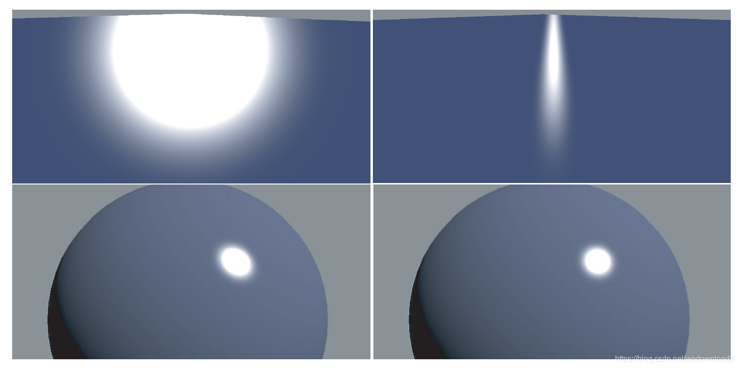
figure 4: on the left, we see two scenes rendered with the original Phong shading model. on the right, we see the same scenes rendered with the Blinn-Phong model. although the differences are subtle on the bottom row (sphere), they are very noticeable on the top row (flat plane). (image from “real-time rendering, 3rd edition” used with permission from A K Peters).

let us now focus on the specular term. what is the physical meaning of the dot product between the reflected view vector and the light? it does not seem to correspond to anything from microfacet theory. Blinn’s modification[2] to the Phong model (typically referred to as the Blinn-Phong model) is very similar to Equation 3, but it uses the more physically meaningful half-vector. recall (from the background talk): the half-vector is the direction to which the microfacet normals m need be oriented to reflect l into v (see figure 3)——the reflection vector has no such physical significance. changing from Phong to Blinn-Phong gives us the following model:

although Blin-Phong is more physically meaningful than the original Phong, it is valid to ask whether this makes any practical difference for production shading. figure 4 compares the visual appearance of the two models. for round objects the two are similar, but for lights glancing off flat surfaces like floors, they are very different. phong has a round highlight and blinn-phong has an elongated thin highlight. if we compare to real-world photographs (figure 5) then it is clear that blinn-phong is much more realistic.

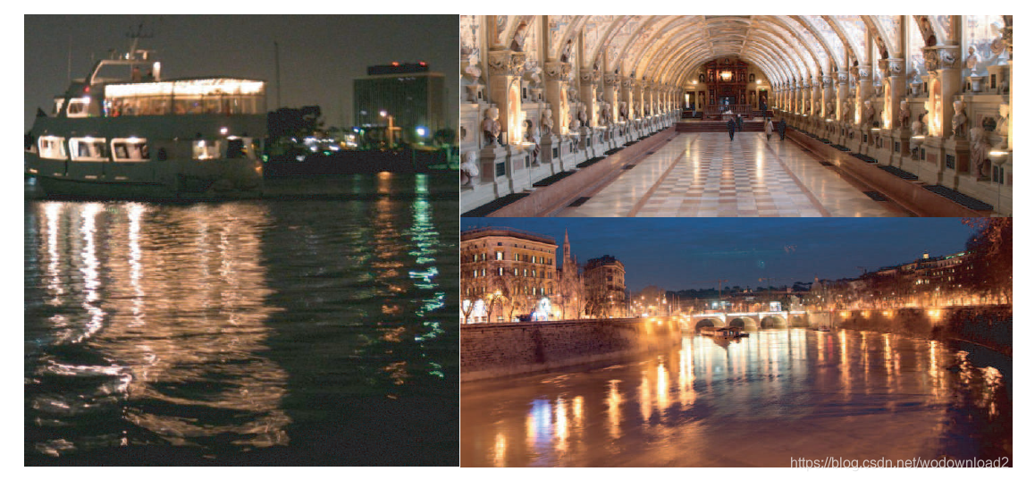
figure 5: the real word displays elongated thin highlights, similar to those predicted by the Blinn-Phong model and very different from those predicted by the original Phong model. (photographs from “real-time rendering, 3rd edition” used with permission from A K Perters and the photographer, Elan Ruskin).

so far using microfacet theory to improve our game shading model has been successful. let us try some more microfacet theory, starting by comparing our current shading model with a microfacet BRDF model lit by a puntual light source:

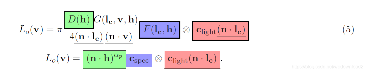
there appear to already be several important similarities; we have highlighted the parts that correspond most closely with matching colors. what are the minimal changes required to turn our model into a full-fledged 完全合格的 microfacet BRDF?

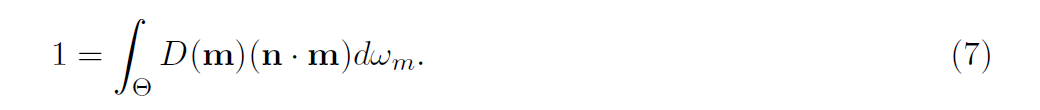
first, we see that the cosine power term already resembles a microfacet distribution funtion evaluated with m=h. however, to convert the cosine power term into a microfacet distribution function it must be correctly normalized. any microfacet distribution needs to fulfill the requirement that the sum of the microfacet areas is equal to the macrosurface area. more precisely, the sum of the signed projected areas of the microfacets needs to equal the signed projected area of the macroscopic surface; this must hold true for any viewing direction [37]. mathematically, this means that the function must fulfil this equation for any v:

note that the integral is over the entire sphere, not just the hemisphere, and the cosine factors are not clamped. this equation holds for any kind of microsurface, not just heightfields. in the special case, v = n:

the Blinn-Phong cosine power term can be made to obey this equation by multiplying it with a simple normalization factor:

这里D的下标BP是blinn-phong的缩写。

the next term that needs to be modified is Cspec. as we saw in the background talk, although the specular reflectance of a given material stays almost constant over a wide range of directions, it always goes to 100% white at a extremely glancing angles. this effect can be simply modeled by replacing Cspec with Fschlick(Cspec, l, h) (the background talk course notes give more details on the schlick approimation). not all games use a constant Cspec as in our example “game shading model”. many games do use the Schlick approximation for Fresnel, but unfortunately it is often used incorrectly. the most common error is to use the Schlick equation to interpolate a scalar “Fresnel factor” to 1 instead of interpolating Cspec to 1. this interpolated “Fresnel factor” is then multiplied with Cspec. this is bad for several reasons. instead of interpolating the surface specular color to white at the edges, this “Fresnel term” instead darkens it at the center. the artist has to specify the edge color instead of the much more intuitive center color, and in the case of colored specular there is no way to get the correct result. worse still, the superfluous “Fresnel factor” parameter is added to the ones the artist needs to manipulate, sometimes even stored per-pixel in a texture, wasting storage space. it is true that this “Fresnel model” is slightly cheapter to compute than the correct one, but given the lack of realism and the awkwardness for the artist, the tiny performance difference is not worth it.

another common error is to use the wrong angle for the Fresnel term. both environment maps and specular highlights require that the specular color be modified by a Fresnel term, but it is not the same term in both cases. the appropriate angle to use when computing environment map Fresnel is the one between n and v, while the angle to use for specular highlight Fresnel is the one between l and h (or equivalently, between v and h). this is because specular highlights are reflected by microfacets with surface normals equal to h. either out of unfamiliarity with the underlying theory or out of temptation to save a few cycles, it is common for developers to use the angle between n and v for both environment map Fresnel and specular highlight Fresnel. this temptation should be resisted——when this angle is uesd for specular highlight Fresnel, any surface which is glancing to the view direction will receive brightened highlights regardless of light direction. this will lead to overly bright highlights throughout the scene, often forcing the use of some hack factor to darken the highlights back down and dooming any chance of achieving realistic specular reflectance.

looking back at Equation 5, we see that part of the microfacet model has no corresponding term in our modified game specular model. this “orphan term” is the shadowing/masking, or geometry term G(Lc, v, h) divided by the “foreshortening factors” (n.lc)(n.v). we refer to this ratio as the visibility term since it combines factors accounting for microfacet self-occlusion and foreshortening. since our modified specular model has no visibility term, we will simply set it to 1. this is the same as setting the geometry term to be equal to the product of the two foreshortening factors, definining the following implicit geometry term:

this is actually a plausible geometry term for a heightfield microsurface (which is what the Blinn-Phong normal distribution function cooresponds to, since it is zero for all backfacing microfacets). Gimplicit() is equal to 1 when l = n and v = n,which is correct for a heightfield (no microfacets areoccluded from the direction of the macrosurface normal). It goes to 0 for either glancing view angles
or glancing light angles, which again is correct (the probability of a microfacet being occluded by other microfacets increases with viewing angle, going to 100% in the limit). Given that this geometry factor actually costs less than zero shader cycles to compute (it cancels out the foreshortening factors so we don’t need to divide by them), it has very good “bang per buck”.

when comparing Gimplicit() to other geometry terms from the literature, we find that it goes to 0 too quickly- it is slightly too dark at moderately glancing angles. in other words, adding a more accurate geometry factor will have the result of somewhat brightening the specular term.

if we plug all these terms (Schlick Fresnel approximation, correctly normalized Blinn-Phong normal distribution function, and implicit geometry term) into the microfacet BRDF in equation 5, we get the following shading model:

Environmental and Ambient light
Environment maps (typically cube maps in game development) are important when using physical shading models. Since they have no diffuse color, all exposed metal surfaces should use environment maps, but it is worth considering using them everywhere, even on “matte” 粗糙的 surfaces. The exact content of the environment map typically does not matter. with a few exceptions (such as a racing game where there is a smooth curved object in the center of the player’s attention), incorrectly-shaped reflections are rarely noticed by players. However, it is important for the average color and intensity of the environment map to match 匹配 the diffuse ambient or indirect lighting, otherwise the material’s appearance will chagne. if both are derived from local samples in the game level (typically precomputed), then they will match by default.

However, it is much easier to vary diffuse ambient lighting continuously over the game environment than to do the same for environment maps. for this reason a way to “track” the environment map to the diffuse ambient is useful. this can be done in a straightforward manner by “normalizing” the environment map (dividing it by its average value) in a pre-process, and then mulitiplying it by the diffuse ambient in the shader. the diffuse ambient value used should be averaged over all normal directions, in the case of spherical harmonics this would be the 0-order SH coefficient. this can produce quite good results even if the original environment map does not contain an image of the level or even of the same game (e.g., real-world light probes can be used).

Shading with environment maps is reasonably straightforward. the same Cspec value uesd for specular highlights should be applied, albeit with a slightly different Fresnel factor.