【AI】PyTorch入门(二):训练与预测
1、AI训练、预测步骤
采集数据
标注数据
加载数据
预处理数据
创建模型
训练——优化模型参数
保存模型及参数
加载模型及参数
预测
2、采集数据
以图像处理为例,获取需要的图像数据,将它们缩放成需要的分辨率,分辨率大小和所创建的模型有关。
3、标注数据
在有监督的机器学习中,一般会对图片做以下处理:
如果是检测,需要标记检测物在图片中的坐标、大小;
如果是分类,将不同类别的图片放入不同的文件夹中。
4、加载数据
PyTorch 提供特定领域的库,例如:处理文本数据处理库TorchText、 图像数据处理库TorchVision和音频波形处理库TorchAudio。所有这些库都包含数据集,例如TorchVision中的datasets可以下载 CIFAR、COCO、FashionMNIST 等数据集。
我们以FashionMNIST为例。
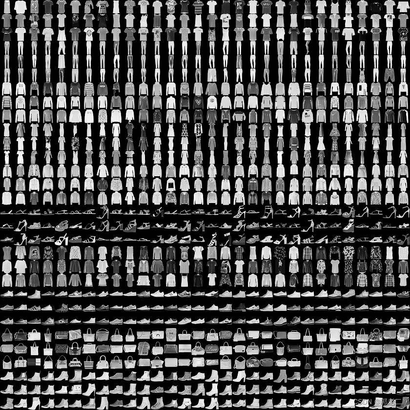
Fashion-MNIST:替代MNIST手写数字集的图像数据集,该数据集由衣服、鞋子等服饰组成,包含70000张图像,其中60000张训练图像加10000张测试图像,图像大小为28x28,单通道,共分10个类,如下图,每三行为一类。
# 导入库
import torch
from torch import nn
from torch.utils.data import DataLoader
from torchvision import datasets
from torchvision.transforms import ToTensor

# 训练集
training_data = datasets.FashionMNIST(
    root="data",
    train=True,
    download=True,
    transform=ToTensor(),
)
#测试集
test_data = datasets.FashionMNIST(
    root="data",
    train=False,
    download=True,
    transform=ToTensor(),
)
幸运的话,会打印下载信息,如下所示:
Downloading http://fashion-mnist.s3-website.eu-central-1.amazonaws.com/train-images-idx3-ubyte.gz
Downloading http://fashion-mnist.s3-website.eu-central-1.amazonaws.com/train-images-idx3-ubyte.gz to data\FashionMNIST\raw\train-images-idx3-ubyte.gz
100.0%
Extracting data\FashionMNIST\raw\train-images-idx3-ubyte.gz to data\FashionMNIST\raw

Downloading http://fashion-mnist.s3-website.eu-central-1.amazonaws.com/train-labels-idx1-ubyte.gz
Downloading http://fashion-mnist.s3-website.eu-central-1.amazonaws.com/train-labels-idx1-ubyte.gz to data\FashionMNIST\raw\train-labels-idx1-ubyte.gz
100.0%
Extracting data\FashionMNIST\raw\train-labels-idx1-ubyte.gz to data\FashionMNIST\raw

Downloading http://fashion-mnist.s3-website.eu-central-1.amazonaws.com/t10k-images-idx3-ubyte.gz
Downloading http://fashion-mnist.s3-website.eu-central-1.amazonaws.com/t10k-images-idx3-ubyte.gz to data\FashionMNIST\raw\t10k-images-idx3-ubyte.gz
100.0%
Extracting data\FashionMNIST\raw\t10k-images-idx3-ubyte.gz to data\FashionMNIST\raw

Downloading http://fashion-mnist.s3-website.eu-central-1.amazonaws.com/t10k-labels-idx1-ubyte.gz
Downloading http://fashion-mnist.s3-website.eu-central-1.amazonaws.com/t10k-labels-idx1-ubyte.gz to data\FashionMNIST\raw\t10k-labels-idx1-ubyte.gz
100.0%
Extracting data\FashionMNIST\raw\t10k-labels-idx1-ubyte.gz to data\FashionMNIST\raw
5、预处理数据
# 每批次大小设为64
batch_size = 64

# 将 torchvision.datasets 交给 torch.utils.data.DataLoader 处理
train_dataloader = DataLoader(training_data, batch_size=batch_size)
test_dataloader = DataLoader(test_data, batch_size=batch_size)

#  N代表数量, C代表channel,H代表高度,W代表宽度
for X, y in test_dataloader:
    print(f"Shape of X [N, C, H, W]: {X.shape}")
    print(f"Shape of y: {y.shape} {y.dtype}")
    break
输出
Shape of X [N, C, H, W]: torch.Size([64, 1, 28, 28])
Shape of y: torch.Size([64]) torch.int64
N代表数量-每批次64张图片;
C代表channel-单通道;
H代表高度、W代表宽度,对应分辨率28*28
6、创建模型
# 如果GPU可用,将数据导入GPU上
device = "cuda" if torch.cuda.is_available() else "cpu"
print(f"Using {device} device")

# 从torch.nn.Module的类,nn.Module 是 PyTorch 体系下所有神经网络模块的基类
class NeuralNetwork(nn.Module):
    def __init__(self):
        super(NeuralNetwork, self).__init__()
        # torch.nn.flatten是一个类,作用为将连续的几个维度展平成一个tensor
        self.flatten = nn.Flatten()
        #  用于定义 linear_relu_stack,由多层神经网络构成;
        # Sequential 意为其下定义的多层操作一个接一个按顺序进行,把它们前后全部拼接在一起。
        self.linear_relu_stack = nn.Sequential(
        	# nn.Linear 是全连接层,28 * 28 表示输入维度数量,512 表示下一层输出数量
            nn.Linear(28*28, 512),
            # ReLU:激活函数
            nn.ReLU(),
            nn.Linear(512, 512),
            nn.ReLU(),
            nn.Linear(512, 10)
        )

	# 向前传播
    def forward(self, x):
        x = self.flatten(x)
        logits = self.linear_relu_stack(x)
        return logits

model = NeuralNetwork().to(device)
print(model)
打印信息
Using cpu device
# 打印网络结构
NeuralNetwork(
  (flatten): Flatten(start_dim=1, end_dim=-1)
  (linear_relu_stack): Sequential(
    (0): Linear(in_features=784, out_features=512, bias=True)
    (1): ReLU()
    (2): Linear(in_features=512, out_features=512, bias=True)
    (3): ReLU()
    (4): Linear(in_features=512, out_features=10, bias=True)
  )
)
关于激活函数:
如果不用激励函数(其实相当于激励函数是f(x) = x),在这种情况下你每一层节点的输入都是上层输出的线性函数,很容易验证,无论你神经网络有多少层,输出都是输入的线性组合,与没有隐藏层效果相当,这种情况就是最原始的感知机(Perceptron)了,那么网络的逼近能力就相当有限。正因为上面的原因,需要引入非线性函数作为激励函数,这样深层神经网络表达能力就更加强大(不再是输入的线性组合,而是几乎可以逼近任意函数)。
7、训练——优化模型参数
定义损失函数和优化器
# loss_fn:损失函数,计算实际输出和真实相差多少;
# CrossEntropyLoss:交叉熵损失函数,做图片分类任务时常用的损失函数。
loss_fn = nn.CrossEntropyLoss()

# optimizer:优化器,用来训练时候优化模型参数
# SGD:表示随机梯度下降,用于控制实际输出y与真实y之间的相差有多大
optimizer = torch.optim.SGD(model.parameters(), lr=1e-3)
训练函数,基本流程是:预测、计算误差、梯度置0、反向传播、优化参数
def train(dataloader, model, loss_fn, optimizer):
    size = len(dataloader.dataset)
    # 训练模式
    model.train()
    for batch, (X, y) in enumerate(dataloader):
        X, y = X.to(device), y.to(device)

        # 获取预测结果
        pred = model(X)
        # 计算预测误差
        loss = loss_fn(pred, y)

        # 优化器工作之前先将梯度置0,进行归零操作
        optimizer.zero_grad()
        # 反向传播
        loss.backward()
        # 优化参数
        optimizer.step()

		# 每100次打印一次信息
        if batch % 100 == 0:
        	# loss 值越低越好,预测值与真实值越来越靠近,这说明模型设计成功
            loss, current = loss.item(), batch * len(X)
            print(f"loss: {loss:>7f}  [{current:>5d}/{size:>5d}]")
评估函数
def test(dataloader, model, loss_fn):
    size = len(dataloader.dataset)
    num_batches = len(dataloader)
    # 评估模式
    model.eval()
    test_loss, correct = 0, 0
    with torch.no_grad():
        for X, y in dataloader:
            X, y = X.to(device), y.to(device)
            pred = model(X)
            test_loss += loss_fn(pred, y).item()
            correct += (pred.argmax(1) == y).type(torch.float).sum().item()
    test_loss /= num_batches
    correct /= size
    print(f"Test Error: \n Accuracy: {(100*correct):>0.1f}%, Avg loss: {test_loss:>8f} \n")
开始迭代训练、评估
# 迭代训练五次
epochs = 5
for t in range(epochs):
    print(f"Epoch {t+1}\n-------------------------------")
    train(train_dataloader, model, loss_fn, optimizer)
    test(test_dataloader, model, loss_fn)
print("Done!")
打印信息
Epoch 1
-------------------------------
loss: 2.298977  [    0/60000]
loss: 2.287373  [ 6400/60000]
loss: 2.271695  [12800/60000]
loss: 2.266561  [19200/60000]
loss: 2.257005  [25600/60000]
loss: 2.214672  [32000/60000]
loss: 2.223222  [38400/60000]
loss: 2.189051  [44800/60000]
loss: 2.183618  [51200/60000]
loss: 2.148876  [57600/60000]
Test Error:
 Accuracy: 41.0%, Avg loss: 2.148859
略...
Epoch 5
-------------------------------
loss: 1.321847  [    0/60000]
略...
loss: 1.059822  [57600/60000]
Test Error:
 Accuracy: 64.3%, Avg loss: 1.081540
Done!
8、保存模型及参数
保存模型的常用方法是序列化模型及参数。将模型和参数保存到文件中。
torch.save(model.state_dict(), "model.pth")
9、加载模型及参数
import torch
from torch import nn
from torchvision.transforms import ToTensor

class NeuralNetwork(nn.Module):
    def __init__(self):
        super(NeuralNetwork, self).__init__()
        # torch.nn.flatten是一个类,作用为将连续的几个维度展平成一个tensor
        self.flatten = nn.Flatten()
        #  用于定义 linear_relu_stack,由多层神经网络构成;
        # Sequential 意为其下定义的多层操作一个接一个按顺序进行,把它们前后全部拼接在一起。
        self.linear_relu_stack = nn.Sequential(
        	# nn.Linear 是全连接层,28 * 28 表示输入维度数量,512 表示下一层输出数量
            nn.Linear(28*28, 512),
            # ReLU:激活函数
            nn.ReLU(),
            nn.Linear(512, 512),
            nn.ReLU(),
            nn.Linear(512, 10)
        )

modelRun = NeuralNetwork()
modelRun.load_state_dict(torch.load("model.pth"))
加载成功,将会输出打印信息,大意是序列化文件中的模型及参数可以加载到运行模型中。
<All keys matched successfully>
10、预测
FashionMNIST数据集标注为0~9,数字对应的服装名称定义在classes中
classes = [
    "T-shirt/top",
    "Trouser",
    "Pullover",
    "Dress",
    "Coat",
    "Sandal",
    "Shirt",
    "Sneaker",
    "Bag",
    "Ankle boot",
]

# 加载评估模型
modelRun.eval()
# 从测试集中获取一张图片及对应的标签,例如获取第六张图片,下标为5
x, y = test_data[5][0], test_data[5][1]
print(f'x.shape =  "{x.shape}" ')
print(f'y=  "{y}" ')

# 预测时,不会向后传播、梯度更新,只会向前推理(no_grad)
with torch.no_grad():
    pred = modelRun(x)
    print(f'pred=  "{pred}" ')
    # 得到预测类别中最高的那一类,再把最高的这一类对应 classes 中的哪一个标签。
    predicted, actual = classes[pred[0].argmax(0)], classes[y]
    print(f'Predicted: "{predicted}", Actual: "{actual}"')
输出结果
x.shape =  "torch.Size([1, 28, 28])"
y=  "1"
pred=  "tensor([[ 2.1079,  3.4801,  0.4381,  2.6778,  1.0602, -2.3333,  0.9451, -3.2445,
     -1.9010, -3.4177]])"
Predicted: "Trouser", Actual: "Trouser"