【R语言文本挖掘】:主题模型(LDA)
【R语言数据科学】
- 🌸个人主页:JOJO数据科学
- 📝个人介绍:统计学top3高校统计学硕士在读
- 💌如果文章对你有帮助,欢迎✌
关注、👍点赞、✌收藏、👍订阅专栏- ✨本文收录于【R语言数据科学】本系列主要介绍R语言在数据科学领域的应用包括:
R语言编程基础、R语言可视化、R语言进行数据操作、R语言建模、R语言机器学习算法实现、R语言统计理论方法实现。本系列会坚持完成下去,请大家多多关注点赞支持,一起学习~,尽量坚持每周持续更新,欢迎大家订阅交流学习!

文章目录
- 【R语言数据科学】
- 主题模型(LDA)
- 1.隐含狄利克雷分布 (LDA)
- 1.1主题词概率
- 1.2 文档-主题概率
- 2.案例:图书主题分类
- 2.1对章节进行主题建模
- 2.2 按文档分类
- 2.3 数据增强:augment
- 3.总结
主题模型(LDA)
在文本挖掘中,我们经常有文档集合,例如博客文章或新闻文章,我们希望将它们分成自然组,以便我们可以分别理解它们。主题模型是一种对此类文档进行无监督分类的方法,类似于对数值型数据进行聚类。
潜在狄利克雷分配 (LDA) 是一种特别流行的拟合主题模型的方法。它将每个文档视为主题的混合,并将每个主题视为单词的混合。这允许文档在内容方面相互“重叠”,而不是被分成离散的组,以反映自然语言的典型使用方式。
在这一章中,我们将学习如何使用topicmodels包中的LDA方法,特别是对这类模型进行整理,使其可以用ggplot2和dplyr进行操作。
1.隐含狄利克雷分布 (LDA)
是一种主题模型,它可以将文档集中每篇文档的主题按照概率分布的形式给出。同时它是一种无监督学习算法,在训练时不需要手工标注的训练集,需要的仅仅是文档集以及指定主题的数量k即可。此外LDA的另一个优点则是,对于每一个主题均可找出一些词语来描述它。主要有以下两个原则:
- 每一个文档包含多个主题.我们设想,每个文档都可能以特定的比例包含几个主题的词。例如,在一个双主题模型中,我们可以说 “文档1是90%的主题A和10%的主题B,而文档2是30%的主题A和70%的主题B。”
- 每一个主题包含多个词.例如,我们可以想象一个美国新闻的双主题模式,一个主题是 “政治”,一个是 “娱乐”。政治话题中最常见的词可能是 “总统”、"国会 "和 “政府”,而娱乐话题可能是由 “电影”、"电视 "和 "演员 "等词组成的。重要的是,不同主题之间可以共享词语;像 "预算 "这样的词语可能同样出现在两个主题中。
这里我们使用AssociatedPress数据集
library(topicmodels)
library(tidyverse)
data("AssociatedPress")
AssociatedPress %>% head()
<<DocumentTermMatrix (documents: 6, terms: 10473)>>
Non-/sparse entries: 1045/61793
Sparsity           : 98%
Maximal term length: 18
Weighting          : term frequency (tf)
我们可以使用topicmodels包中的LDA()函数,设置k=2,来创建一个双主题的LDA模型。
在实践中,几乎所有的主题模型都会使用较大的k,但我们很快就会看到,这种分析方法可以延伸到更多的主题。
此函数返回一个对象,其中包含模型拟合的全部详细信息,例如单词如何与主题相关联以及主题如何与文档相关联。
ap_lda <- LDA(AssociatedPress, k = 2, control = list(seed = 2022))
ap_lda
A LDA_VEM topic model with 2 topics.
1.1主题词概率
library(tidytext)
ap_topics <- tidy(ap_lda, matrix = "beta")#使用tidy函数,选择beta得到各个主题下,单词的概率值
ap_topics %>% head()
| topic | term | beta |
|---|---|---|
| <int> | <chr> | <dbl> |
| 1 | aaron | 3.086419e-05 |
| 2 | aaron | 1.162187e-05 |
| 1 | abandon | 1.068572e-05 |
| 2 | abandon | 6.834240e-05 |
| 1 | abandoned | 1.213616e-04 |
| 2 | abandoned | 4.948278e-05 |
此时的数据是一个主题一个单词的概率值,接下来我们使用在之前介绍过的slice_max()来观察每个主题下出现平常最多的是歌词
library(ggplot2)
ap_top_terms <- ap_topics %>%
 group_by(topic) %>% # 分组聚合
 slice_max(beta,n=10) %>%# 每一个主题下最出现频次最多的10个词
 ungroup %>%# 取消分组
 arrange(topic,-beta)#降序排序
ap_top_terms %>% head()
| topic | term | beta |
|---|---|---|
| <int> | <chr> | <dbl> |
| 1 | i | 0.007210257 |
| 1 | people | 0.005597826 |
| 1 | two | 0.004640735 |
| 1 | police | 0.004226899 |
| 1 | years | 0.003494558 |
| 1 | government | 0.003384736 |
ap_top_terms %>%
  mutate(term = reorder_within(term, beta, topic)) %>%#重新排序
  ggplot(aes(beta, term, fill = factor(topic))) +
  geom_col(show.legend = FALSE) +
  facet_wrap(~ topic, scales = "free") +
  scale_y_reordered()
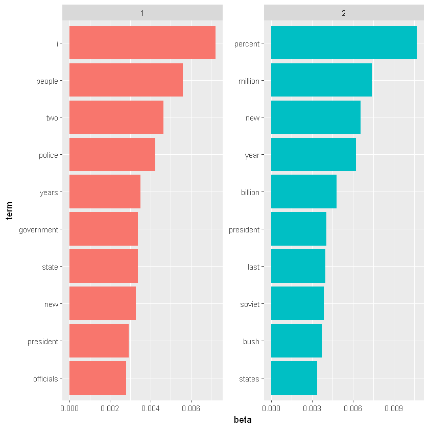
这种可视化让我们了解从文章中提取的两个主题。主题2中最常见的词包括 “百分比”、“百万”、"亿 "和 “公司”,这表明它可能代表商业或金融新闻。主题1中最常见的词包括 “总统”、“政府”,这表明该主题代表政治新闻。关于每个主题中的词语的一个重要观察是,一些词语,如 "new"和 “president”,在两个话题中都很常见。这是主题建模相对于 "聚类 "方法的一个优势:自然语言中使用的话题在词语方面可能有一些重叠。作为一个替代方案,我们可以考虑那些在以下方面差异最大的词语。我们考虑使用对数比率来进行比较, l o g ( β 1 β 2 ) log(\frac{\beta_1}{\beta_2}) log(β2β1)
beta_wide <- ap_topics %>%
  mutate(topic = paste0("topic", topic)) %>%
  pivot_wider(names_from = topic, values_from = beta) %>%#将数据转换为宽数据格式
  filter(topic1 > .001 | topic2 > .001) %>%
  mutate(log_ratio = log2(topic2 / topic1))
beta_wide %>% head()
| term | topic1 | topic2 | log_ratio |
|---|---|---|---|
| <chr> | <dbl> | <dbl> | <dbl> |
| administration | 4.863621e-04 | 0.001712912 | 1.81634804 |
| agreement | 2.272349e-04 | 0.001832509 | 3.01156333 |
| aid | 2.350136e-04 | 0.001208183 | 2.36202222 |
| air | 1.064362e-03 | 0.001037106 | -0.03742491 |
| american | 1.378128e-03 | 0.002467178 | 0.84015190 |
| analysts | 4.797704e-11 | 0.001087046 | 24.43349355 |
1.2 文档-主题概率
除了估计每个主题词的概率外,LDA还将每个文档看做是很多主题的集合。我们可以检查每个文档每个主题的概率,称为
γ(“gamma”),使用tidy()的matrix = "gamma "参数。
ap_documents <- tidy(ap_lda, matrix = "gamma")
ap_documents%>%head()
| document | topic | gamma |
|---|---|---|
| <int> | <int> | <dbl> |
| 1 | 1 | 0.9992228 |
| 2 | 1 | 0.5084786 |
| 3 | 1 | 0.9991869 |
| 4 | 1 | 0.7855420 |
| 5 | 1 | 0.9968537 |
| 6 | 1 | 0.5899276 |
这些值中的每一个都是该文档中由该主题产生的词的估计比例。例如,我们可以看到,许多文档是来自两个主题的混合,但是文档1几乎完全来自于主题1
tidy(AssociatedPress) %>%
  filter(document == 1) %>%
  arrange(desc(count)) %>%head()
| document | term | count |
|---|---|---|
| <int> | <chr> | <dbl> |
| 1 | police | 7 |
| 1 | school | 7 |
| 1 | teacher | 7 |
| 1 | shot | 5 |
| 1 | students | 5 |
| 1 | boy | 4 |
可以看出包含警察、学校、老师、射击、学生。这可能是一个关于校园恐怖事件的新闻
2.案例:图书主题分类
在检查统计方法时,在你知道“正确答案”的情况下尝试它会很有用。例如,我们可以收集一组3个完全独立主题的文档,然后进行主题建模,看看算法是否能正确区分这3个组。这让我们可以仔细检查该方法是否有用,并了解它如何以及何时会出错。我们将使用一些经典文献中的数据来尝试这一点。
假设我们有四本书,但是被一个破坏者撕毁了,但是这里假设我们知道这四本书如下:
- Great Expectations by Charles Dickens
- Twenty Thousand Leagues Under the Sea by Jules Verne
- Pride and Prejudice by Jane Austen
这个破坏者把这些书撕成单独的章节,然后把它们堆成一大堆。我们如何才能将这些杂乱无章的章节恢复到原来的书中?这是一个具有挑战性的问题,因为各个章节没有标签:我们不知道哪些词可以将它们区分为组。因此,我们将使用主题建模来发现章节如何聚集成不同的主题,每个主题(可能)代表一本书。
book_name <- c("Twenty Thousand Leagues under the Sea",
            "Pride and Prejudice",
            "Great Expectations")
library(gutenbergr)

books <- gutenberg_works(title %in% book_name) %>%
  gutenberg_download(meta_fields = "title")
首先对数据进行预处理,我们把这些内容分成章节,使用tidytext的unnest_tokens()把它们分成单词,然后删除stop_words。我们把每一章都当作一个独立的 “文档”,每章都有一个名字,比如《远大前程》_1或者《傲慢与偏见》_1。(在其他应用中,每个文档可能是一篇报纸文章,或一篇博客文章)。
library(stringr)

# 将书分成文档,每一个文档代表一章
by_chapter <- books %>%
  group_by(title) %>%
  mutate(chapter = cumsum(str_detect(
    text, regex("^chapter ", ignore_case = TrUE)
  ))) %>%
  ungroup() %>%
  filter(chapter > 0) %>%
  unite(document, title, chapter)

# 分词处理
by_chapter_word <- by_chapter %>%
  unnest_tokens(word, text)

# 将停用词去除,并且记数
word_counts <- by_chapter_word %>%
  anti_join(stop_words) %>%
  count(document, word, sort = TrUE)
[1m[22mJoining, by = "word"
word_counts%>%head()
| document | word | n |
|---|---|---|
| <chr> | <chr> | <int> |
| Great Expectations_57 | joe | 88 |
| Great Expectations_7 | joe | 70 |
| Great Expectations_17 | biddy | 63 |
| Great Expectations_27 | joe | 58 |
| Great Expectations_38 | estella | 58 |
| Great Expectations_2 | joe | 56 |
2.1对章节进行主题建模
首先,使用cast_dtm函数将数据进行转换成一个文档矩阵
chapters_dtm <- word_counts %>%
  cast_dtm(document, word, n)
chapters_dtm
<<DocumentTermMatrix (documents: 166, terms: 16535)>>
Non-/sparse entries: 90679/2654131
Sparsity           : 97%
Maximal term length: 19
Weighting          : term frequency (tf)
然后我们就可以使用LDA函数进行主题模型的拟合,这里k取3,因为我们有三本书
chapters_lda <- LDA(chapters_dtm, k = 3, control = list(seed = 2022))
chapters_lda
A LDA_VEM topic model with 3 topics.
同样,我们可以得到每一个主题下每一个单词的概率
chapter_topics <- tidy(chapters_lda, matrix = "beta")
chapter_topics %>% head()
| topic | term | beta |
|---|---|---|
| <int> | <chr> | <dbl> |
| 1 | joe | 4.291604e-09 |
| 2 | joe | 1.254313e-95 |
| 3 | joe | 1.255518e-02 |
| 1 | biddy | 1.715859e-10 |
| 2 | biddy | 9.449672e-240 |
| 3 | biddy | 4.136679e-03 |
请注意,这已将模型转换为每行一个主题的格式。对于每个组合,模型都会计算从该主题生成该术语的概率。例如,“joe”这个词从主题 1、2 生成的概率几乎为零,但它占主题 3 的 2%。
和之前一样,使用slice_max()函数找出每一个主题下出现频次最多的5个单词
top_terms <- chapter_topics %>%
    group_by(topic) %>%
    slice_max(beta,n=5) %>%
    ungroup() %>%
    arrange(topic, -beta)
top_terms %>% head()
| topic | term | beta |
|---|---|---|
| <int> | <chr> | <dbl> |
| 1 | elizabeth | 0.015125588 |
| 1 | darcy | 0.009466182 |
| 1 | miss | 0.007707367 |
| 1 | bennet | 0.007486658 |
| 1 | jane | 0.007004467 |
| 2 | captain | 0.015262393 |
top_terms %>%
  mutate(term = reorder_within(term, beta, topic)) %>%
  ggplot(aes(beta, term, fill = factor(topic))) +
  geom_col(show.legend = FALSE) +
  facet_wrap(~ topic, scales = "free") +
  scale_y_reordered()

这些主题与这四本书明显相关!毫无疑问,“船长”、“鹦鹉螺”、“海”和“尼莫”的话题属于海底两万里,而“简”、“达西”和“伊丽莎白”属于《傲慢和偏见》。我们在 Great Expectations 中看到“pip”和“joe”。我们还注意到,由于 LDA 是一种“模糊聚类”方法,多个主题之间可以有共同的词,例如主题1和3的miss
2.2 按文档分类
在这次分析中,每份文档都代表一个章节。因此,我们可能想知道哪些主题与这些文档有关。我们能不能把这些章节重新组合到正确的书中?我们可以通过检查每个文档-每个主题的概率来发现这一点。在这里使用γ(“gamma”)。
chapters_gamma <- tidy(chapters_lda, matrix = "gamma")
chapters_gamma %>% head()
| document | topic | gamma |
|---|---|---|
| <chr> | <int> | <dbl> |
| Great Expectations_57 | 1 | 1.935895e-01 |
| Great Expectations_7 | 1 | 3.100871e-01 |
| Great Expectations_17 | 1 | 9.056126e-02 |
| Great Expectations_27 | 1 | 6.215130e-02 |
| Great Expectations_38 | 1 | 5.063431e-02 |
| Great Expectations_2 | 1 | 1.832306e-05 |
现在我们有了这些主题概率,我们可以看看我们的无监督学习在区分这三本书方面做得如何。我们期望一本书中的章节会被发现大部分(或全部)是由相应的主题产生的。
首先,我们把文档名称重新分为标题和章节,然后我们可以直观地看到每个文档每个主题的概率
chapters_gamma <- chapters_gamma %>%
  separate(document, c("title", "chapter"), sep = "_", convert = TrUE)

chapters_gamma %>% head()
| title | chapter | topic | gamma |
|---|---|---|---|
| <chr> | <int> | <int> | <dbl> |
| Great Expectations | 57 | 1 | 1.935895e-01 |
| Great Expectations | 7 | 1 | 3.100871e-01 |
| Great Expectations | 17 | 1 | 9.056126e-02 |
| Great Expectations | 27 | 1 | 6.215130e-02 |
| Great Expectations | 38 | 1 | 5.063431e-02 |
| Great Expectations | 2 | 1 | 1.832306e-05 |
chapters_gamma %>%
  mutate(title = reorder(title, gamma * topic)) %>%
  ggplot(aes(factor(topic), gamma)) +
  geom_boxplot() +
  facet_wrap(~ title) +
  labs(x = "topic", y = expression(gamma))
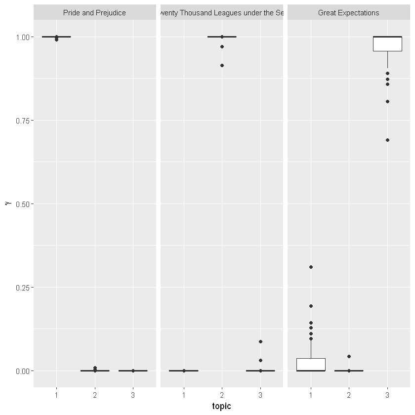
我们注意到,《傲慢与偏见》、和《海底两万里》几乎所有章节都被唯一标识为一个主题。
看起来《远大前程》中的某些章节(应该是主题3)与其他主题有些关联。是否存在与章节最相关的主题属于另一本书的情况?首先,我们将使用 slice_max() 找到与每一章最相关的主题
chapter_classifications <- chapters_gamma %>%
  group_by(title, chapter) %>%
  slice_max(gamma) %>%
  ungroup()

chapter_classifications%>%head()
| title | chapter | topic | gamma |
|---|---|---|---|
| <chr> | <int> | <int> | <dbl> |
| Great Expectations | 1 | 3 | 0.9999296 |
| Great Expectations | 2 | 3 | 0.9999634 |
| Great Expectations | 3 | 3 | 0.9999310 |
| Great Expectations | 4 | 3 | 0.9425210 |
| Great Expectations | 5 | 3 | 0.9999683 |
| Great Expectations | 6 | 3 | 0.9998279 |
chapter_classifications <- chapters_gamma %>%
  group_by(title, chapter) %>%
  slice_max(gamma) %>%
  ungroup()
chapter_classifications %>%head()
| title | chapter | topic | gamma |
|---|---|---|---|
| <chr> | <int> | <int> | <dbl> |
| Great Expectations | 1 | 3 | 0.9999296 |
| Great Expectations | 2 | 3 | 0.9999634 |
| Great Expectations | 3 | 3 | 0.9999310 |
| Great Expectations | 4 | 3 | 0.9425210 |
| Great Expectations | 5 | 3 | 0.9999683 |
| Great Expectations | 6 | 3 | 0.9998279 |
然后,我们可以将每个主题与每本书的“共识”主题(其章节中最常见的主题)进行比较,看看哪些主题最常被错误识别。
book_topics <- chapter_classifications %>%
  count(title, topic) %>%
  group_by(title) %>%
  slice_max(n, n = 1) %>%
  ungroup() %>%
  transmute(consensus = title, topic)

chapter_classifications %>%
  inner_join(book_topics, by = "topic") %>%
  filter(title != consensus)
| title | chapter | topic | gamma | consensus |
|---|---|---|---|---|
| <chr> | <int> | <int> | <dbl> | <chr> |
我们看到没有错误分类的,这对于无监督聚类算法而言,结果还算不错!
2.3 数据增强:augment
LDA 算法的一个步骤是将每个文档中的每个单词分配给一个主题。文档中分配给该主题的单词越多,通常,该文档-主题分类的权重 (gamma) 就越大。我们可能想要获取原始文档-单词对并找出每个文档中的哪些单词被分配给了哪个主题。这是 augment() 函数的工作,它也起源于 broom 包,作为整理模型输出的一种方式。 tidy() 检索模型的统计组件,而 augment() 使用模型将信息添加到原始数据中的每个观察值。
assignments <- augment(chapters_lda, data = chapters_dtm)
assignments%>%head()
| document | term | count | .topic |
|---|---|---|---|
| <chr> | <chr> | <dbl> | <dbl> |
| Great Expectations_57 | joe | 88 | 3 |
| Great Expectations_7 | joe | 70 | 3 |
| Great Expectations_17 | joe | 5 | 3 |
| Great Expectations_27 | joe | 58 | 3 |
| Great Expectations_2 | joe | 56 | 3 |
| Great Expectations_23 | joe | 1 | 3 |
这将返回一个整洁的书籍术语计数数据框,但添加了一个额外的列:.topic,其中每个术语在每个文档中分配给了主题。 (通过 augment 添加的额外列始终以 . 开头,以防止覆盖现有列)。我们可以将此分配表与共识书名相结合,以找出哪些单词被错误分类。
assignments <- assignments %>%
  separate(document, c("title", "chapter"),
           sep = "_", convert = TrUE) %>%
  inner_join(book_topics, by = c(".topic" = "topic"))

assignments%>%head()
| title | chapter | term | count | .topic | consensus |
|---|---|---|---|---|---|
| <chr> | <int> | <chr> | <dbl> | <dbl> | <chr> |
| Great Expectations | 57 | joe | 88 | 3 | Great Expectations |
| Great Expectations | 7 | joe | 70 | 3 | Great Expectations |
| Great Expectations | 17 | joe | 5 | 3 | Great Expectations |
| Great Expectations | 27 | joe | 58 | 3 | Great Expectations |
| Great Expectations | 2 | joe | 56 | 3 | Great Expectations |
| Great Expectations | 23 | joe | 1 | 3 | Great Expectations |
真正的书(title)和分配给它的书(consensus)的这种组合对于进一步探索很有用。例如,我们可以使用 dplyr 的 count() 和 ggplot2 的 geom_tile 可视化一个混淆矩阵,显示一本书中的单词分配给另一本书的频率。
library(scales)

assignments %>%
  count(title, consensus, wt = count) %>%
  mutate(across(c(title, consensus), ~str_wrap(., 20))) %>%
  group_by(title) %>%
  mutate(percent = n / sum(n)) %>%
  ggplot(aes(consensus, title, fill = percent)) +
  geom_tile() +
  scale_fill_gradient2(high = "darkred", label = percent_format()) +
  theme_minimal() +
  theme(axis.text.x = element_text(angle = 90, hjust = 1),
        panel.grid = element_blank()) +
  labs(x = "Book words were assigned to",
       y = "Book words came from",
       fill = "% of assignments")
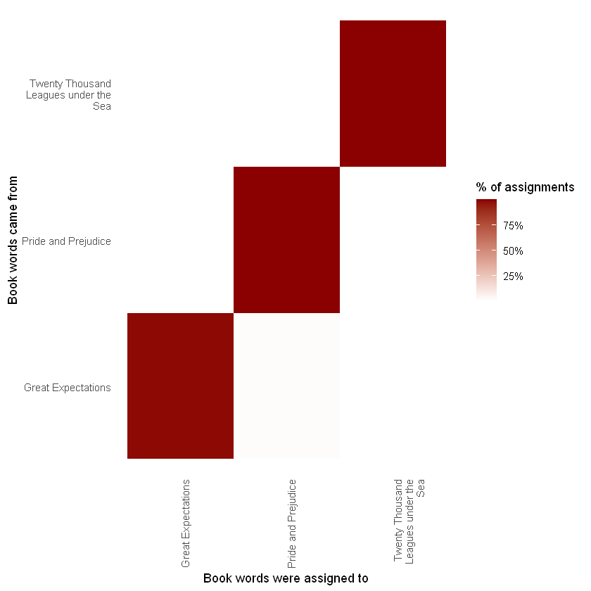
我们注意到《傲慢与偏见》、《海底两万里》中几乎所有的词都被正确分配了,而《远大前程》有相当多的错误分配的词,我们再来看一下哪些是最容易分类错误的词
wrong_words <- assignments %>%
  filter(title != consensus)
wrong_words%>%head()
| title | chapter | term | count | .topic | consensus |
|---|---|---|---|---|---|
| <chr> | <int> | <chr> | <dbl> | <dbl> | <chr> |
| Twenty Thousand Leagues under the Sea | 8 | miss | 1 | 3 | Great Expectations |
| Pride and Prejudice | 9 | captain | 1 | 2 | Twenty Thousand Leagues under the Sea |
| Pride and Prejudice | 7 | captain | 3 | 2 | Twenty Thousand Leagues under the Sea |
| Great Expectations | 54 | sea | 2 | 2 | Twenty Thousand Leagues under the Sea |
| Pride and Prejudice | 41 | sea | 1 | 2 | Twenty Thousand Leagues under the Sea |
| Great Expectations | 7 | lady | 1 | 1 | Pride and Prejudice |
wrong_words %>%
  count(title, consensus, term, wt = count) %>%
  ungroup() %>%
  arrange(desc(n)) %>% head()
| title | consensus | term | n |
|---|---|---|---|
| <chr> | <chr> | <chr> | <dbl> |
| Great Expectations | Pride and Prejudice | jane | 13 |
| Great Expectations | Pride and Prejudice | uncle | 11 |
| Great Expectations | Pride and Prejudice | aunt | 10 |
| Great Expectations | Pride and Prejudice | letter | 8 |
| Great Expectations | Pride and Prejudice | marriage | 8 |
| Great Expectations | Pride and Prejudice | hart | 7 |
我们可以看到,即使出现在《远大前程》中,很多词也经常被分配到傲慢与偏见中。对于其中一些词,例如“爱”和“女士”,这是因为它们在《傲慢与偏见》中更为常见(我们可以通过检查计数来确认)。
另一方面,有一些错误分类的词从未出现在小说中,它们被错误分配。例如,我们可以确认“flopson”仅出现在 Great Expectations 中,即使它被分配到“傲慢与偏见”集群中。
word_counts %>%
  filter(word == "flopson")
| document | word | n |
|---|---|---|
| <chr> | <chr> | <int> |
| Great Expectations_22 | flopson | 10 |
| Great Expectations_23 | flopson | 7 |
| Great Expectations_33 | flopson | 1 |
LDA 算法是随机的,它可能会意外地落在跨越多本书的主题上。
3.总结
本章介绍了用于查找表征一组文档的词簇的主题建模,并展示了 tidy() 动词如何让我们使用 dplyr 和 ggplot2 探索和理解这些模型。这是模型探索 tidy 方法的优势之一:不同输出格式的挑战由整理功能处理,我们可以使用一组标准工具来探索模型结果。特别是,我们看到主题建模能够从三本书中分离和区分章节,并通过查找错误分配的单词和章节来探索模型的局限性。
🔎本章的介绍到此介绍,如果文章对你有帮助,请多多点赞、收藏、评论、关注支持!!