空间域:空间组学的耶路撒冷
文章目录
- 环境配置与数据
- Squidpy
- SpaGCN
- 将基因表达和组织学整合到一个图上
- 基因表达数据质控与预处理
- SpaGCN的超参
- 优化空间域
- 参考文献
空间组学不能没有空间域,就如同蛋白质不能没有结构域。
摘要:
- 空间域是反映细胞在基因表达方面的相似性以及空间邻近性的簇
- 识别空间域的方法也可以通过空间组学技术纳入可用的组织学信息
- 使用Squidpy和SpaGCN识别空间域
完整Notebook版本代码:https://github.com/grassdream/Spatial-Omics/blob/main/spatial_domain.ipynb
生物信息学就是和数据打交道,我们就是要从数据中挖掘出有用信息,寻找特定的模式。我们有了空间组学数据,就是想着要从中寻找出随空间变化的模式,空间域–Spatial Domain就是其中最重要的模式之一。间组学不能没有空间域,就如同蛋白质不能没有结构域一般。
空间组学的数据主要包括两大部分:细胞x基因矩阵和空间坐标。此外还有一些附加信息,比如细胞的类型和大小,以及对应的组织学图像等等。
目前有很多识别空间域的算法,基本上可以分为两类:①基于空间远近的基因表达的相似度聚类;②联合组织学图像。
空间远近:
- Spatial domains in Squidpy [Palla et al., 2022]
- Hidden-Markov random field (HMRF) [Dries et al., 2021]
- BayesSpace [Zhao et al., 2021]
联合组织学图像:
- spaGCN [Hu et al., 2021]
- stLearn [Pham et al., 2020]
下面我们来看看到底怎么识别空间域吧!
环境配置与数据
安装自不必说,这里我们设置sc.settings.verbosity = 3,verbosity是唠叨、冗长的意思,我们设置这个唠叨级别为3,这样Scanpy会在运行过程中输出更多的信息和警告,帮助用户更好地了解正在发生的事情。
Level 0: only show ‘error’ messages.
Level 1: also show ‘warning’ messages.
Level 2: also show ‘info’ messages.
Level 3: also show ‘hint’ messages.
Level 4: also show very detailed progress for ‘debug’ging.
# !pip install scanpy
# !pip install squidpy
import scanpy as sc
import squidpy as sqsc.settings.verbosity = 3
# 设置Scanpy的输出详细程度的命令。详细程度为3时,Scanpy会在运行过程中输出更多的信息和警告,帮助用户更好地了解正在发生的事情。
sc.settings.set_figure_params(dpi=80, facecolor="white")
# 设置图形参数的命令。这里设置了图形的dpi(图像清晰度)为80,以及图形的背景颜色为白色。
我们选择的数据是Squidypy预处理的数据,这是由10x Genomics Space Ranger 1.1.0提供的来自一只小鼠的一个组织切片。
既然是预处理的,我们直接加载即可。
https://squidpy.readthedocs.io/en/stable/api/squidpy.datasets.visium_hne_adata.html
# adata = sq.datasets.visium_hne_adata()
# https://ndownloader.figshare.com/files/26098397
# 报错的话自己下载读取即可
# https://scanpy.readthedocs.io/en/stable/generated/scanpy.read_h5ad.html
adata = sc.read_h5ad("../data/visium_hne.h5ad")
adata
AnnData object with n_obs × n_vars = 2688 × 18078obs: 'in_tissue', 'array_row', 'array_col', 'n_genes_by_counts', 'log1p_n_genes_by_counts', 'total_counts', 'log1p_total_counts', 'pct_counts_in_top_50_genes', 'pct_counts_in_top_100_genes', 'pct_counts_in_top_200_genes', 'pct_counts_in_top_500_genes', 'total_counts_mt', 'log1p_total_counts_mt', 'pct_counts_mt', 'n_counts', 'leiden', 'cluster'var: 'gene_ids', 'feature_types', 'genome', 'mt', 'n_cells_by_counts', 'mean_counts', 'log1p_mean_counts', 'pct_dropout_by_counts', 'total_counts', 'log1p_total_counts', 'n_cells', 'highly_variable', 'highly_variable_rank', 'means', 'variances', 'variances_norm'uns: 'cluster_colors', 'hvg', 'leiden', 'leiden_colors', 'neighbors', 'pca', 'rank_genes_groups', 'spatial', 'umap'obsm: 'X_pca', 'X_umap', 'spatial'varm: 'PCs'obsp: 'connectivities', 'distances'
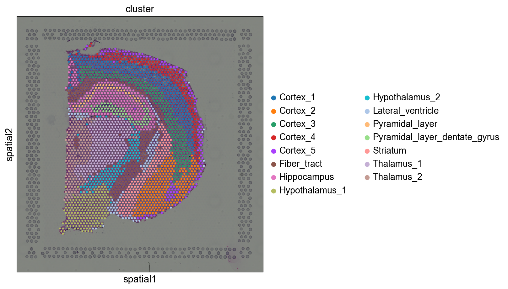
这是预处理的数据,我们看看预处理的cluster的情况。
我们使用sq.pl.spatial_scatter()函数,它可以在组织图像的背景上绘制数据的空间分布,也可以只绘制数据的散点图。
sq.pl.spatial_scatter(adata, color="cluster", figsize=(10, 10))
/exampleminiconda3/envs/GNN/lib/python3.10/site-packages/squidpy/pl/_spatial_utils.py:483: FutureWarning: The default value of 'ignore' for the `na_action` parameter in pandas.Categorical.map is deprecated and will be changed to 'None' in a future version. Please set na_action to the desired value to avoid seeing this warningcolor_vector = color_source_vector.map(color_map)
Squidpy
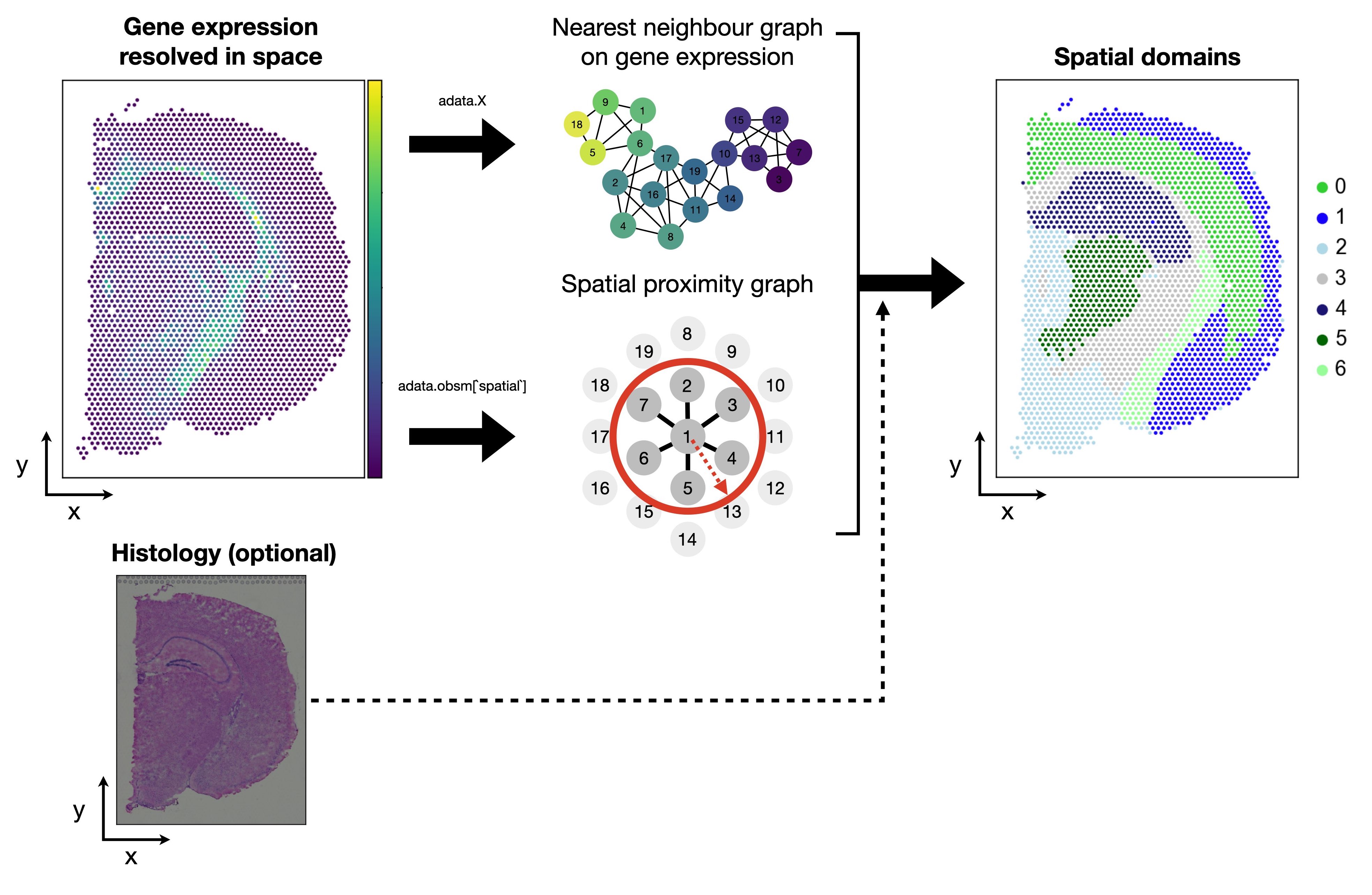
首先,我们要在两个不同的空间上计算spot之间的相似性,一个是基因表达空间,一个是空间坐标。为了表示这种相似性,我们可以用最近邻图(也就是空间上的邻居网络)来构建数据点之间的连接关系。
下面的代码用到了adata.obsm['X_pca'],这是数据里已经有的,之后我会从原始数据出发的,敬请关注。
# nearest neighbor graph
sc.pp.neighbors(adata)
nn_graph_genes = adata.obsp["connectivities"]
# spatial proximity graph
sq.gr.spatial_neighbors(adata)
nn_graph_space = adata.obsp["spatial_connectivities"]
computing neighborsusing 'X_pca' with n_pcs = 502024-01-29 19:05:12.156250: W tensorflow/stream_executor/platform/default/dso_loader.cc:64] Could not load dynamic library 'libcudart.so.11.0'; dlerror: libcudart.so.11.0: cannot open shared object file: No such file or directory
2024-01-29 19:05:12.156343: I tensorflow/stream_executor/cuda/cudart_stub.cc:29] Ignore above cudart dlerror if you do not have a GPU set up on your machine.finished: added to `.uns['neighbors']``.obsp['distances']`, distances for each pair of neighbors`.obsp['connectivities']`, weighted adjacency matrix (0:00:18)
Creating graph using `grid` coordinates and `None` transform and `1` libraries.
Adding `adata.obsp['spatial_connectivities']``adata.obsp['spatial_distances']``adata.uns['spatial_neighbors']`
Finish (0:00:00)
第二部,我们要同时考虑两个空间上的相似性,然后来识别数据中的社区(community)或者聚类(cluster)。
一个简单的方法是把两个最近邻图相加,得到一个联合的最近邻图(joint graph),然后在这个图上运行 leiden 算法。leiden 算法是一种基于模块度(modularity)优化的社区检测算法,它可以把数据点划分为不同的社区,使得同一社区内的数据点相似度高,不同社区间的数据点相似度低。
我们还可以用一个超参数 alpha 来调节两个空间上的相似性的重要性。alpha 的值越大,表示空间坐标上的相似性越重要,反之,基因表达上的相似性越重要。这里,我们设置 alpha = 0.2,表示我们更倾向于基于基因表达的相似性。
因此,我们可以用下面的公式来计算联合的最近邻图:
alpha = 0.2
joint_graph = (1 - alpha) * nn_graph_genes + alpha * nn_graph_space
最后,我们用 sc.tl.leiden 函数来在联合的最近邻图上运行 leiden 算法,得到数据点的社区划分,并把结果保存在 adata 对象的 squidpy_domains 属性中。
sc.tl.leiden(adata, adjacency=joint_graph, key_added="squidpy_domains")
running Leiden clusteringfinished: found 17 clusters and added'squidpy_domains', the cluster labels (adata.obs, categorical) (0:00:00)
让我们来看看识别的空间域和最开始的cluster之间的相似程度吧!
由于要画两个图,我们就要设置子图间距,调节wspace即可。
- wspace指定了子图之间的水平间距,单位是轴的宽度的百分比1。
- wspace值越大,表示子图之间的水平间距越大,反之,子图之间的水平间距越小。
- 默认值是 0.2,表示子图之间的水平间距是轴的宽度的 20%1。
- 这里,我们设置 wspace = 0.9,表示我们想要增加子图之间的水平间距,使得子图更清晰地分开。
sq.pl.spatial_scatter(adata, color=["cluster", "squidpy_domains"], wspace=0.9)
/example/miniconda3/envs/GNN/lib/python3.10/site-packages/squidpy/pl/_spatial_utils.py:483: FutureWarning: The default value of 'ignore' for the `na_action` parameter in pandas.Categorical.map is deprecated and will be changed to 'None' in a future version. Please set na_action to the desired value to avoid seeing this warningcolor_vector = color_source_vector.map(color_map)
/example/miniconda3/envs/GNN/lib/python3.10/site-packages/squidpy/pl/_spatial_utils.py:483: FutureWarning: The default value of 'ignore' for the `na_action` parameter in pandas.Categorical.map is deprecated and will be changed to 'None' in a future version. Please set na_action to the desired value to avoid seeing this warningcolor_vector = color_source_vector.map(color_map)
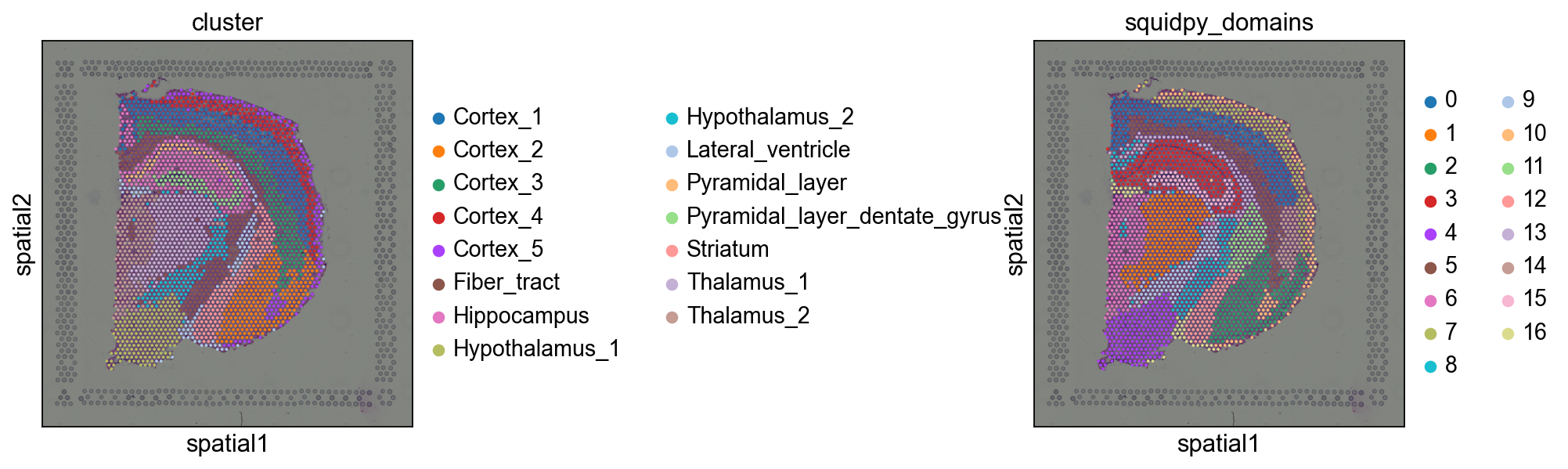
我们可以看到,这种方法本质上是基于空间距离“平滑”聚类注释。尽管这是一种纯粹的教学方法,但它已在实践中使用[Chen et al.,2022]。
SpaGCN
SpaGCN是一种利用基因表达、空间位置和组织学进行空间组学数据分析的图卷积神经网络方法。
SpaGCN在无向加权图中结合了基因表达、空间信息和组织学图像。这个图可以表示数据中存在的整体空间依赖关系,然后就可用图卷积来识别空间域。
# !pip install SpaGCN
import SpaGCN as spgimport numpy as np
from PIL import Image
import requests
前面提到了,SpaGCN利用了额外的组织学图像数据。我们就通过request从10x Genomics网站上加载高分辨率的tif文件。
不过SpaGCN也可以不利用组织学信息,我们等会儿再说。
img = np.asarray(Image.open(requests.get("https://cf.10xgenomics.com/samples/spatial-exp/1.1.0/V1_Adult_Mouse_Brain/V1_Adult_Mouse_Brain_image.tif",stream=True,).raw)
)
/example/miniconda3/envs/GNN/lib/python3.10/site-packages/PIL/Image.py:3157: DecompressionBombWarning: Image size (132748287 pixels) exceeds limit of 89478485 pixels, could be decompression bomb DOS attack.warnings.warn(
我们的anndata数据是经过预处理的,SpaGCN是需要原始数据的,所以我们就重置adata.X。
将基因表达和组织学整合到一个图上
SpaGCN需要把spatial array的坐标和pixel的坐标传入模型。前者存放在 adata.obs["array_row"] 和 adata.obs["array_col"],后者存放在adata.obsm["spatial"]。
# Set coordinates
x_array = adata.obs["array_row"].tolist()
y_array = adata.obs["array_col"].tolist()
x_pixel = (adata.obsm["spatial"][:, 0]).tolist()
y_pixel = adata.obsm["spatial"][:, 1].tolist()
SpaGCN首先把基因表达和组织学信息以邻接矩阵的形式整合到一张图上。两个点相连的条件是物理上里的很近并且又相似的组织学特征。下面就是对应的函数了,除了需要输入坐标,还有两个参数:
beta决定了在提取color intensity是每个spot的面积。这个值通常来说存储在adata.uns['spatial]。Visium spot一般是55~100 μ m \mu m μm。alpha决定了在计算点之间的欧式距离时给组织学图像的权重。alpha=1表示组织学像素强度值与(x,y)坐标具有相同的scale cariance。
# Calculate adjacent matrix
adj = spg.calculate_adj_matrix(x=x_pixel,y=y_pixel,x_pixel=x_pixel,y_pixel=y_pixel,image=img,beta=55,alpha=1,histology=True,
)
Calculateing adj matrix using histology image...
Var of c0,c1,c2 =  96.93674686223055 519.0133178897761 37.20274924909862
Var of x,y,z =  2928460.011122931 4665090.578837907 4665090.578837907
基因表达数据质控与预处理
接下来就是基因表达数据的常规操作了,过滤掉只在不足3个spot中表达的基因。然后把counts进行标准化和对数转换。
adata.var_names_make_unique()sc.pp.filter_genes(adata, min_cells=3)# find mitochondrial (MT) genes
adata.var["MT_gene"] = [gene.startswith("MT-") for gene in adata.var_names]
# remove MT genes (keeping their counts in the object)
adata.obsm["MT"] = adata[:, adata.var["MT_gene"].values].X.toarray()
adata = adata[:, ~adata.var["MT_gene"].values].copy()# Normalize and take log for UMI
sc.pp.normalize_total(adata)
sc.pp.log1p(adata)
normalizing counts per cellfinished (0:00:00)
SpaGCN的超参
第一步,SpaGCN找到characteristiv length scale l l l。这个参数决定了权重作为距离函数衰减的速度。要找到 l l l,首先必须指定参数 p p p, p p p描述由邻域贡献占总表达量的百分比。对于Visium数据,SpaGCN建议使用“p=0.5”。对于Slide-seq V2或MERFISH等捕获区域较小的数据,建议选择较高的贡献值。
p = 0.5
# Find the l value given p
l = spg.search_l(p, adj)
Run 1: l [0.01, 1000], p [0.0, 176.04695830342547]
Run 2: l [0.01, 500.005], p [0.0, 38.50406265258789]
Run 3: l [0.01, 250.0075], p [0.0, 7.22906494140625]
Run 4: l [0.01, 125.00874999999999], p [0.0, 1.119886875152588]
Run 5: l [62.509375, 125.00874999999999], p [0.07394278049468994, 1.119886875152588]
Run 6: l [93.7590625, 125.00874999999999], p [0.4443991184234619, 1.119886875152588]
Run 7: l [93.7590625, 109.38390625], p [0.4443991184234619, 0.7433689832687378]
Run 8: l [93.7590625, 101.571484375], p [0.4443991184234619, 0.5843360424041748]
Run 9: l [93.7590625, 97.66527343749999], p [0.4443991184234619, 0.5119975805282593]
Run 10: l [95.71216796875, 97.66527343749999], p [0.47760796546936035, 0.5119975805282593]
recommended l =  96.688720703125
如果组织中的spatial domain数量是已知的,SpaGCN就可以计算出一个合适的分辨率去生成对应的个数的空间域。一般来说,在大脑样本会这样,比如我们像在切片中找到一定数目的皮层(cortex),如果不给定空间域的个数,那么SpaGCN的分辨率参数就会在0.2到0.1选择具有最高的轮廓系数的值。
在我们的数据中就定为15。
# Search for suitable resolution
res = spg.search_res(adata, adj, l, target_num=15)
Start at res =  0.4 step =  0.1
Initializing cluster centers with louvain, resolution =  0.4
computing neighborsusing data matrix X directlyfinished: added to `.uns['neighbors']``.obsp['distances']`, distances for each pair of neighbors`.obsp['connectivities']`, weighted adjacency matrix (0:00:00)
running Louvain clusteringusing the "louvain" package of Traag (2017)finished: found 9 clusters and added'louvain', the cluster labels (adata.obs, categorical) (0:00:00)
Epoch  0
Res =  0.4 Num of clusters =  9Initializing cluster centers with louvain, resolution =  0.5
computing neighborsusing data matrix X directlyfinished: added to `.uns['neighbors']``.obsp['distances']`, distances for each pair of neighbors`.obsp['connectivities']`, weighted adjacency matrix (0:00:00)
running Louvain clusteringusing the "louvain" package of Traag (2017)finished: found 10 clusters and added'louvain', the cluster labels (adata.obs, categorical) (0:00:00)
Epoch  0
Res =  0.5 Num of clusters =  10
Res changed to 0.5
Initializing cluster centers with louvain, resolution =  0.6
computing neighborsusing data matrix X directlyfinished: added to `.uns['neighbors']``.obsp['distances']`, distances for each pair of neighbors`.obsp['connectivities']`, weighted adjacency matrix (0:00:00)
running Louvain clusteringusing the "louvain" package of Traag (2017)finished: found 11 clusters and added'louvain', the cluster labels (adata.obs, categorical) (0:00:00)
Epoch  0
Res =  0.6 Num of clusters =  11
Res changed to 0.6
Initializing cluster centers with louvain, resolution =  0.7
computing neighborsusing data matrix X directlyfinished: added to `.uns['neighbors']``.obsp['distances']`, distances for each pair of neighbors`.obsp['connectivities']`, weighted adjacency matrix (0:00:00)
running Louvain clusteringusing the "louvain" package of Traag (2017)finished: found 14 clusters and added'louvain', the cluster labels (adata.obs, categorical) (0:00:00)
Epoch  0
Res =  0.7 Num of clusters =  14
Res changed to 0.7
Initializing cluster centers with louvain, resolution =  0.7999999999999999
computing neighborsusing data matrix X directlyfinished: added to `.uns['neighbors']``.obsp['distances']`, distances for each pair of neighbors`.obsp['connectivities']`, weighted adjacency matrix (0:00:00)
running Louvain clusteringusing the "louvain" package of Traag (2017)finished: found 15 clusters and added'louvain', the cluster labels (adata.obs, categorical) (0:00:00)
Epoch  0
Res =  0.7999999999999999 Num of clusters =  15
recommended res =  0.7999999999999999
我们现在已经计算了初始化SpaGCN的所有参数,首先来设置 l l l。
model = spg.SpaGCN()
model.set_l(l)
然后我们开始训练模型,使用我们刚刚找到的分辨率和规定的15个空间域。
model.train(adata, adj, res=res)
Initializing cluster centers with louvain, resolution =  0.7999999999999999
computing neighborsusing data matrix X directlyfinished: added to `.uns['neighbors']``.obsp['distances']`, distances for each pair of neighbors`.obsp['connectivities']`, weighted adjacency matrix (0:00:00)
running Louvain clusteringusing the "louvain" package of Traag (2017)finished: found 14 clusters and added'louvain', the cluster labels (adata.obs, categorical) (0:00:00)
Epoch  0
Epoch  10
Epoch  20
Epoch  30
Epoch  40
Epoch  50
Epoch  60
Epoch  70
delta_label  0.0003720238095238095 < tol  0.001
Reach tolerance threshold. Stopping training.
Total epoch: 73
我们现在就开始预测数据集中每个细胞的空间域。另外模型还会返回细胞属于哪个空间域的概率,不过我们这次暂时用不到。
y_pred, prob = model.predict()
我们把识别的空间域保存到adata.obs并且转换为分类变量,这样方便可视化。
adata.obs["spaGCN_domains"] = y_pred
adata.obs["spaGCN_domains"] = adata.obs["spaGCN_domains"].astype("category")
让我们来和原始的cluster对比一下吧。
sq.pl.spatial_scatter(adata, color=["spaGCN_domains", "cluster"])
/example/miniconda3/envs/GNN/lib/python3.10/site-packages/squidpy/pl/_spatial_utils.py:483: FutureWarning: The default value of 'ignore' for the `na_action` parameter in pandas.Categorical.map is deprecated and will be changed to 'None' in a future version. Please set na_action to the desired value to avoid seeing this warningcolor_vector = color_source_vector.map(color_map)
/example/miniconda3/envs/GNN/lib/python3.10/site-packages/squidpy/pl/_spatial_utils.py:483: FutureWarning: The default value of 'ignore' for the `na_action` parameter in pandas.Categorical.map is deprecated and will be changed to 'None' in a future version. Please set na_action to the desired value to avoid seeing this warningcolor_vector = color_source_vector.map(color_map)
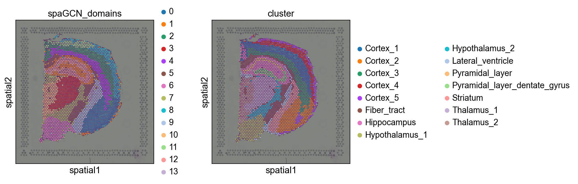
我们可以看到,SpaGCN非常准确地识别了空间域。不过我们可以观察到一些不完美的异常值。SpaGCN提供了一个函数来细化空间域,我们现在来看看这个函数吧。
优化空间域
SpaGCN包括一个可选的改进步骤,以增强聚类结果,这个步骤检查每个点及其相邻点的域分配。如果超过一半的相邻spot被分配到不同的域,则该spot将被重新标记为其相邻spot的主域。细化步骤将只影响几个spot。通常,SpaGCN只建议在数据集期望具有明确的域边界时进行细化。
简单来说就是看看spot的邻居,如果邻居都是A,而它是B,就把B变成A。
这个步骤SpaGCN首先计算邻接矩阵,而不考虑组织学图像。
adj_2d = spg.calculate_adj_matrix(x=x_array, y=y_array, histology=False)
Calculateing adj matrix using xy only...
用邻接矩阵和刚刚识别的空间域来优化。
refined_pred = spg.refine(sample_id=adata.obs.index.tolist(),pred=adata.obs["spaGCN_domains"].tolist(),dis=adj_2d,
)
依然保存,并转换为分类变量。
adata.obs["refined_spaGCN_domains"] = refined_pred
adata.obs["refined_spaGCN_domains"] = adata.obs["refined_spaGCN_domains"].astype("category"
)
我们来看看这三次的识别空间域的结果吧。
sq.pl.spatial_scatter(adata, color=["spaGCN_domains", "refined_spaGCN_domains", "cluster"])
/example/miniconda3/envs/GNN/lib/python3.10/site-packages/squidpy/pl/_spatial_utils.py:483: FutureWarning: The default value of 'ignore' for the `na_action` parameter in pandas.Categorical.map is deprecated and will be changed to 'None' in a future version. Please set na_action to the desired value to avoid seeing this warningcolor_vector = color_source_vector.map(color_map)
/example/miniconda3/envs/GNN/lib/python3.10/site-packages/squidpy/pl/_spatial_utils.py:483: FutureWarning: The default value of 'ignore' for the `na_action` parameter in pandas.Categorical.map is deprecated and will be changed to 'None' in a future version. Please set na_action to the desired value to avoid seeing this warningcolor_vector = color_source_vector.map(color_map)
/example/miniconda3/envs/GNN/lib/python3.10/site-packages/squidpy/pl/_spatial_utils.py:483: FutureWarning: The default value of 'ignore' for the `na_action` parameter in pandas.Categorical.map is deprecated and will be changed to 'None' in a future version. Please set na_action to the desired value to avoid seeing this warningcolor_vector = color_source_vector.map(color_map)
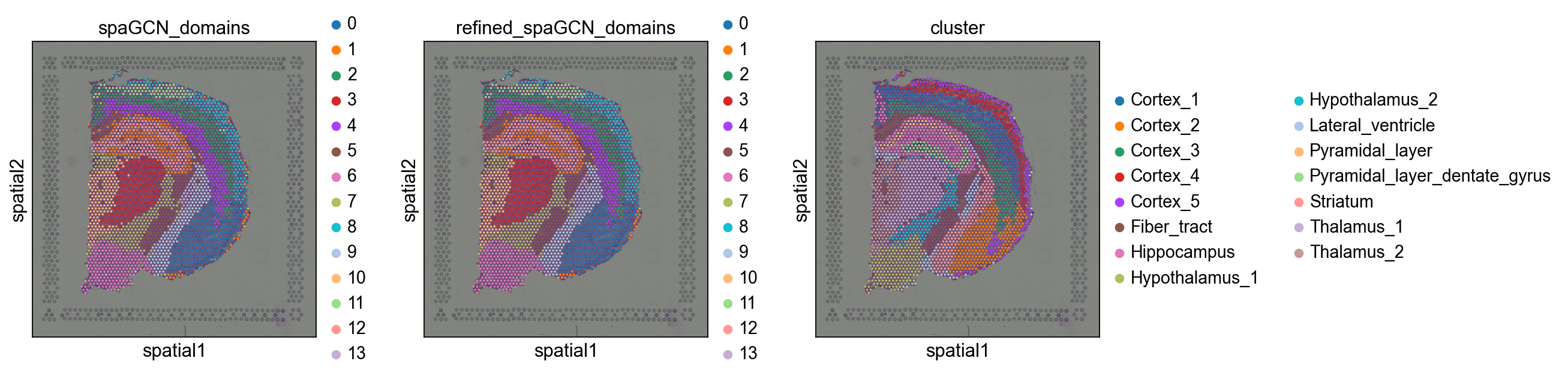
可以看到第一张图的橙色区域的一些异常值就被优化了。
参考文献
https://www.sc-best-practices.org/spatial/domains.html
如果觉得还不错,记得点赞+收藏哟!谢谢大家的阅读!( ̄︶ ̄)↗