数据降维与可视化——t-SNE

t-SNE 是一种数据降维技术，通过把高维的数据降到 2~3维，方便使用可视化技术来展示数据。
论文下载

重要参数：

def tsne(X=np.array([]), no_dims=2, initial_dims=50, perplexity=30.0):

• $X\in R^{N\times D}$ ，N 个样本，每个样本由 D 维数据构成；
• no_dims 压缩后的维度，默认为 2
• init_dims：使用 PCA 对数据预处理，将原始样本集的维度降低至 initial_dims 维度，默认为 30
• perplexity：高斯分布的困惑度，默认为 30；

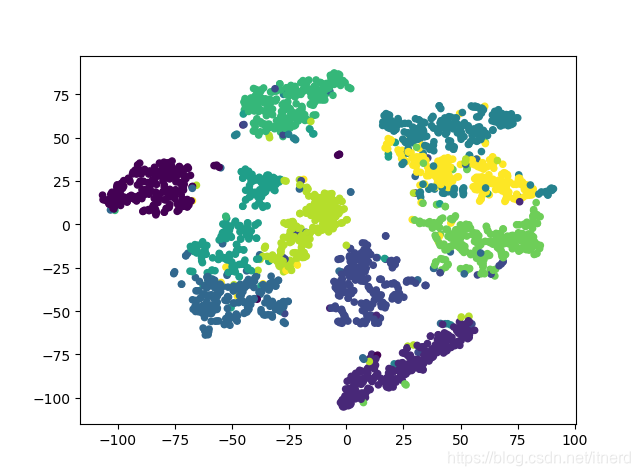
对 MNIST 数据二维可视化

#
#  tsne.py
#
# Implementation of t-SNE in Python. The implementation was tested on Python
# 2.7.10, and it requires a working installation of NumPy. The implementation
# comes with an example on the MNIST dataset. In order to plot the
# results of this example, a working installation of matplotlib is required.
#
# The example can be run by executing: `ipython tsne.py`
#
#
#  Created by Laurens van der Maaten on 20-12-08.
#  Copyright (c) 2008 Tilburg University. All rights reserved.

import numpy as np
import pylab


def Hbeta(D=np.array([]), beta=1.0):
    """
        Compute the perplexity and the P-row for a specific value of the
        precision of a Gaussian distribution.
    """

    # Compute P-row and corresponding perplexity
    P = np.exp(-D.copy() * beta)
    sumP = sum(P)
    H = np.log(sumP) + beta * np.sum(D * P) / sumP
    P = P / sumP
    return H, P


def x2p(X=np.array([]), tol=1e-5, perplexity=30.0):
    """
        Performs a binary search to get P-values in such a way that each
        conditional Gaussian has the same perplexity.
    """

    # Initialize some variables
    print("Computing pairwise distances...")
    (n, d) = X.shape
    sum_X = np.sum(np.square(X), 1)
    D = np.add(np.add(-2 * np.dot(X, X.T), sum_X).T, sum_X)
    P = np.zeros((n, n))
    beta = np.ones((n, 1))
    logU = np.log(perplexity)

    # Loop over all datapoints
    for i in range(n):

        # Print progress
        if i % 500 == 0:
            print("Computing P-values for point %d of %d..." % (i, n))

        # Compute the Gaussian kernel and entropy for the current precision
        betamin = -np.inf
        betamax = np.inf
        Di = D[i, np.concatenate((np.r_[0:i], np.r_[i+1:n]))]
        (H, thisP) = Hbeta(Di, beta[i])

        # Evaluate whether the perplexity is within tolerance
        Hdiff = H - logU
        tries = 0
        while np.abs(Hdiff) > tol and tries < 50:

            # If not, increase or decrease precision
            if Hdiff > 0:
                betamin = beta[i].copy()
                if betamax == np.inf or betamax == -np.inf:
                    beta[i] = beta[i] * 2.
                else:
                    beta[i] = (beta[i] + betamax) / 2.
            else:
                betamax = beta[i].copy()
                if betamin == np.inf or betamin == -np.inf:
                    beta[i] = beta[i] / 2.
                else:
                    beta[i] = (beta[i] + betamin) / 2.

            # Recompute the values
            (H, thisP) = Hbeta(Di, beta[i])
            Hdiff = H - logU
            tries += 1

        # Set the final row of P
        P[i, np.concatenate((np.r_[0:i], np.r_[i+1:n]))] = thisP

    # Return final P-matrix
    print("Mean value of sigma: %f" % np.mean(np.sqrt(1 / beta)))
    return P


def pca(X=np.array([]), no_dims=50):
    """
        Runs PCA on the NxD array X in order to reduce its dimensionality to
        no_dims dimensions.
    """

    print("Preprocessing the data using PCA...")
    (n, d) = X.shape
    X = X - np.tile(np.mean(X, 0), (n, 1))
    (l, M) = np.linalg.eig(np.dot(X.T, X))
    Y = np.dot(X, M[:, 0:no_dims])
    return Y


def tsne(X=np.array([]), no_dims=2, initial_dims=50, perplexity=30.0):
    """
        Runs t-SNE on the dataset in the NxD array X to reduce its
        dimensionality to no_dims dimensions. The syntaxis of the function is
        `Y = tsne.tsne(X, no_dims, perplexity), where X is an NxD NumPy array.
    """

    # Check inputs
    if isinstance(no_dims, float):
        print("Error: array X should have type float.")
        return -1
    if round(no_dims) != no_dims:
        print("Error: number of dimensions should be an integer.")
        return -1

    # Initialize variables
    X = pca(X, initial_dims).real
    (n, d) = X.shape
    max_iter = 1000
    initial_momentum = 0.5
    final_momentum = 0.8
    eta = 500
    min_gain = 0.01
    Y = np.random.randn(n, no_dims)
    dY = np.zeros((n, no_dims))
    iY = np.zeros((n, no_dims))
    gains = np.ones((n, no_dims))

    # Compute P-values
    P = x2p(X, 1e-5, perplexity)
    P = P + np.transpose(P)
    P = P / np.sum(P)
    P = P * 4.									# early exaggeration
    P = np.maximum(P, 1e-12)

    # Run iterations
    for iter in range(max_iter):

        # Compute pairwise affinities
        sum_Y = np.sum(np.square(Y), 1)
        num = -2. * np.dot(Y, Y.T)
        num = 1. / (1. + np.add(np.add(num, sum_Y).T, sum_Y))
        num[range(n), range(n)] = 0.
        Q = num / np.sum(num)
        Q = np.maximum(Q, 1e-12)

        # Compute gradient
        PQ = P - Q
        for i in range(n):
            dY[i, :] = np.sum(np.tile(PQ[:, i] * num[:, i], (no_dims, 1)).T * (Y[i, :] - Y), 0)

        # Perform the update
        if iter < 20:
            momentum = initial_momentum
        else:
            momentum = final_momentum
        gains = (gains + 0.2) * ((dY > 0.) != (iY > 0.)) + \
                (gains * 0.8) * ((dY > 0.) == (iY > 0.))
        gains[gains < min_gain] = min_gain
        iY = momentum * iY - eta * (gains * dY)
        Y = Y + iY
        Y = Y - np.tile(np.mean(Y, 0), (n, 1))

        # Compute current value of cost function
        if (iter + 1) % 10 == 0:
            C = np.sum(P * np.log(P / Q))
            print("Iteration %d: error is %f" % (iter + 1, C))

        # Stop lying about P-values
        if iter == 100:
            P = P / 4.

    # Return solution
    return Y


if __name__ == "__main__":
    print("Run Y = tsne.tsne(X, no_dims, perplexity) to perform t-SNE on your dataset.")
    print("Running example on 2,500 MNIST digits...")
    X = np.loadtxt("mnist2500_X.txt")
    labels = np.loadtxt("mnist2500_labels.txt")
    Y = tsne(X, 2, 50, 20.0)
    pylab.scatter(Y[:, 0], Y[:, 1], 20, labels)
    pylab.show()