AlexNet论文解析—ImageNet Classification with Deep Convolutional Neural Networks
AlexNet论文解析—ImageNet Classification with Deep Convolutional Neural Networks 2012
研究背景
认识数据集:ImageNet的大规模图像识别挑战赛
LSVRC-2012:ImageNet Large Scale Visual Recoanition Challenge
| 类别 | 训练数据 | 测试数据 | 图片格式 | |
|---|---|---|---|---|
| Mnist | 10 | 50000 | 10000 | gray |
| cifar-10 | 10 | 50000 | 10000 | RGB |
| imagenet | 1000 | 1200000 | 150000 | RGB |
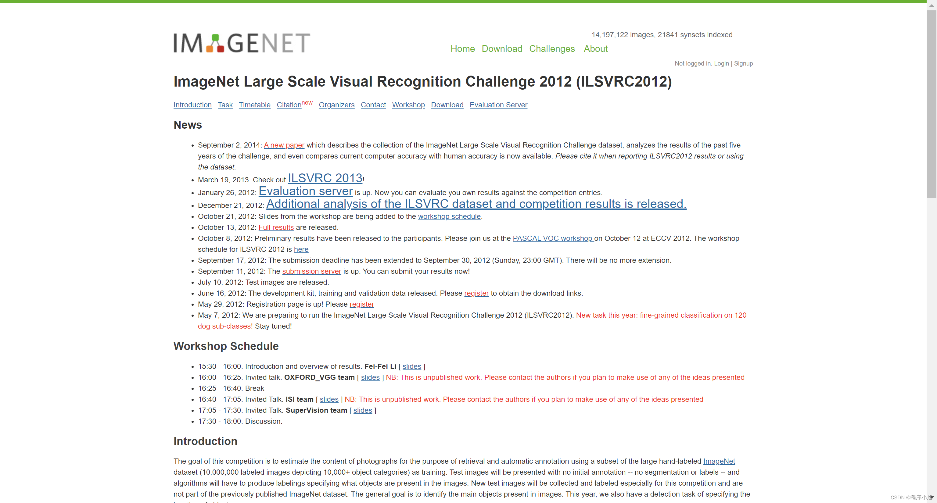
ImageNet Large Scale Visual Recognition Challenge 是李飞飞等人于2010年创办的图像识别挑战赛,自2010起连续举办8年,极大地推动计算机视觉发展。
比赛项目涵盖:图像分类(Classification)、目标定位(Object localization)、目标检测(Object detection)、视频目标检测(Object detection from video)、场景分类(Scene classification)、场景解析(Scene parsing)
竞赛中脱颖而出大量经典模型:
alexnet,vgg,googlenet ,resnet,densenet等
ImageNet数据集包含21841个类别,14,197122张图片其通过WordNet对类别进行分组,使数据集
的语义信息更合理,非常适合图像识别ILSVRC-2012从lmageNet中挑选1000类的1,200,000张作为训练集
在2012年图像分类挑战赛上的评价指标top5 error在任务的介绍中有相关的定义:
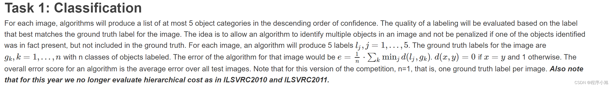
算法要预测出5个类别,要与真实的标签来进行匹配,正确为0,错误为1.在5个比较值当中去最小值来进行计算。
在官网发布的信息中查看比赛的最终结果。
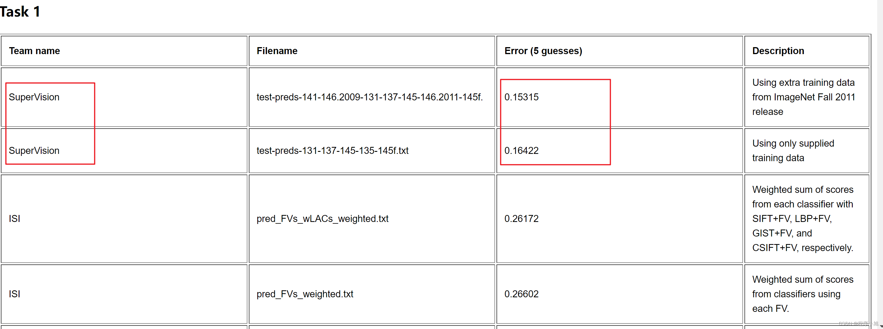
从比赛结果看出第一名的团队的结果领先第二名10%的百分比(深度学习引发了人们的关注)
在训练过程中使用到了强大的计算资源:GPU 580 3G x 2 使得大型的神经网络可以快速的训练
研究成果
AlexNet在ILSVRC-2012L以超出第二名10.9个百分点夺冠
拉开卷积神经网络统治计算机视觉的序幕加速计算机视觉应用落地。从机器学习领域的特征工程到深度学习领域的神经网络
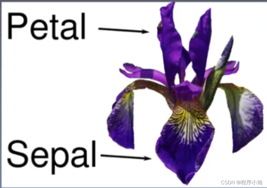
对于常用到的鸢尾花数据集,在机器学习中的处理步骤为:
- 鸢尾花图片
- 特征工程
- 分类模型
- 分类结果
同时开启了相关的应用领域:
安防领域的人脸识别、行人检测、智能视频分析、行人跟踪等,交通领域的交通场景物体识别、车辆计数、逆行检测、车牌检测与识别,以及互联网领域的基于内容的图像检索、相册自动归类等
论文精读
摘要
We trained a large, deep convolutional neural network to classify the 1.2 million high-resolution images in the ImageNet LSVRC-2010 contest into the 1000 different classes. On the test data, we achieved top-1 and top-5 error rates of 37.5% and 17.0% which is considerably better than the previous state-of-the-art. The neural network, which has 60 million parameters and 650,000 neurons, consists of five convolutional layers, some of which are followed by max-pooling layers, and three fully-connected layers with a final 1000-way softmax. To make training faster, we used non-saturating neurons and a very efficient GPU implementation of the convolution operation. To reduce overfitting in the fully-connected
layers we employed a recently-developed regularization method called “dropout” that proved to be very effective. We also entered a variant of this model in the ILSVRC-2012 competition and achieved a winning top-5 test error rate of 15.3%, compared to 26.2% achieved by the second-best entry
摘要进行解读
1.在ILSVRC-2010的120万张图片上训练深度卷积神经网络,获得最优结果,top-1和top-5error分别为37.5%,17%
2.该网络(AlexNet)由5个卷积层和3个全连接层构成,共计6000万参数,65万个神经元
3.为加快训练,采用非饱和激活函数一一ReLU,采用GPU训练
4.为减轻过拟合,采用Dropout
5.基于以上模型及技巧,在ILSVRC-2012以超出第二名10.9个百分点成绩夺冠。
快速的泛读论文,确定文章的小标题结构
- lntroduction
- TheDataset
- TheArchitecture
- 3.1 ReLU Nonlinearity
- 3.2Trainingon Multiple GPUs
- 3.3Local Response Normalization
- 3.4Overlapping Pooling
- 3.5Overall Architecture
- Reducing Overfitting
- 4.1 Data Augmentation
- 4.2Dropout
- Details of learning
- Results
- 6.1QualitativeEvaluations
- Discussion
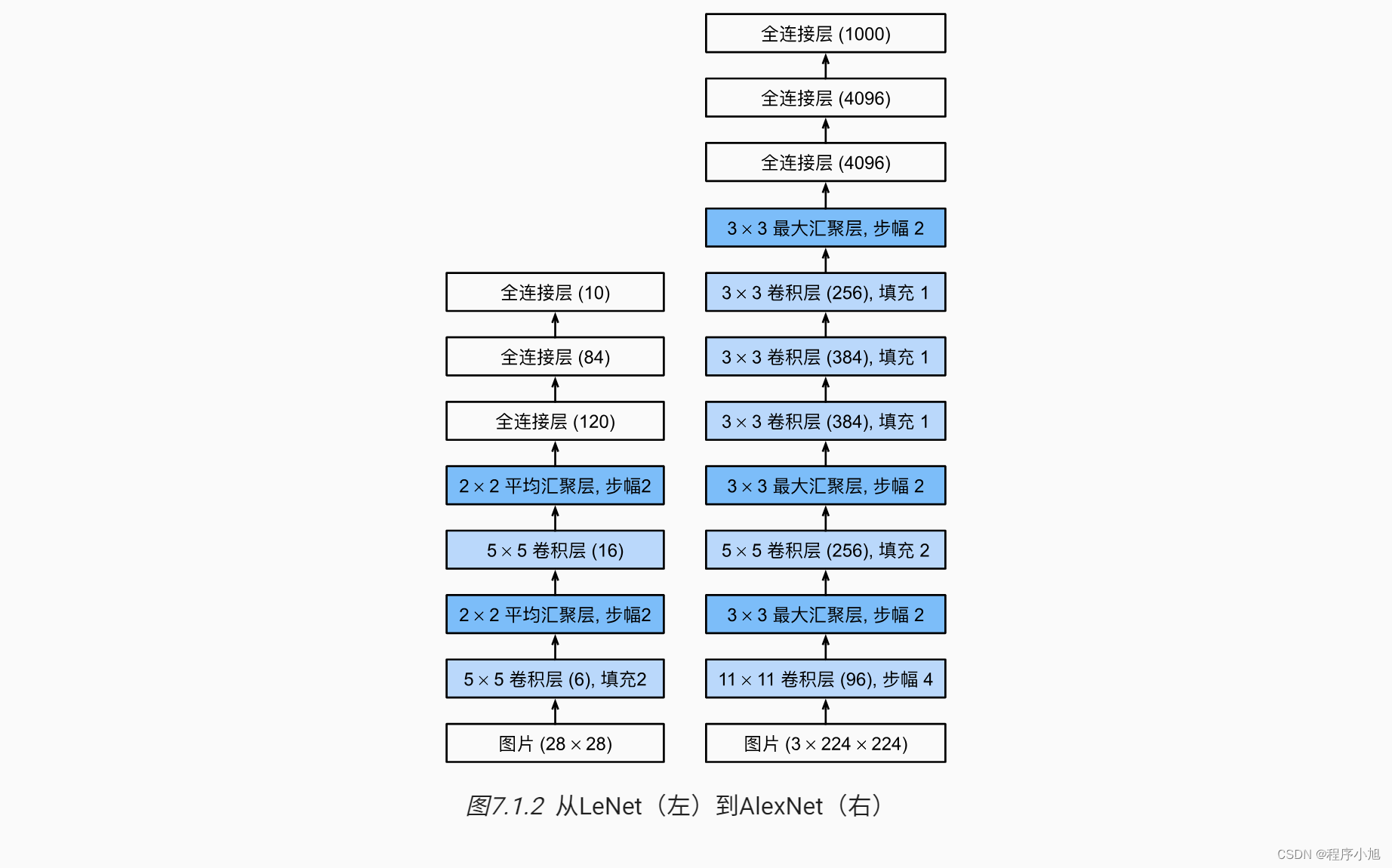
AlexNet网络结构
首先给出论文中的AlexNet的网络结构
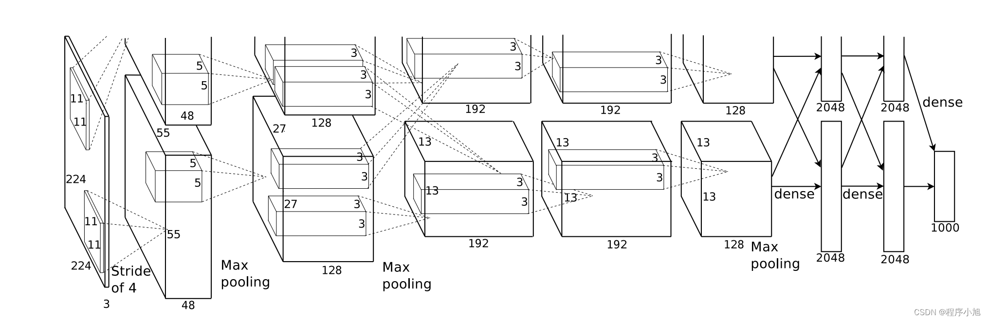
在论文整体的结构解释中可以看出:
As depicted in Figure 2, the net contains eight layers with weights; the first five are convolutional and the remaining three are fullyconnected. The output of the last fully-connected layer is fed to a 1000-way softmax which produces a distribution over the 1000 class labels.
整个alexnet网络分为了8层,包括了前面的5个卷积层,和后面的三个全连接层最后通过softmax函数得到最后的1000分类
使用双GPU来进行训练,每一个块对应一个GPU训练
回顾特征图输出大小的计算公式:
F o = ⌊ F in − k + 2 p s ⌋ + 1 F_{o}=\left\lfloor\frac{F_{\text {in }}-k+2 p}{s}\right\rfloor+1 Fo=⌊sFin −k+2p⌋+1
图中是有一部分省略的若是224 x 224的无填充,经过下取整运算后+1的到的输出,应该是54 x 54的(参考李沐老师案例)
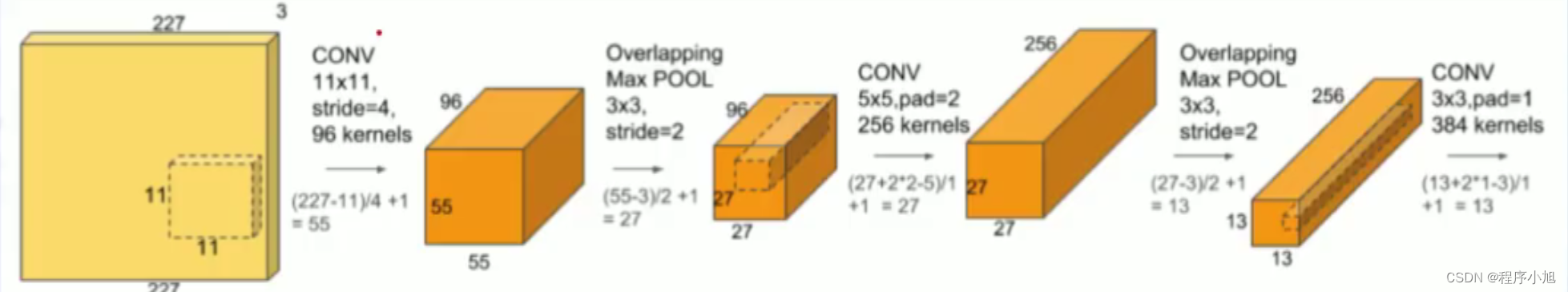
第一层卷积
根据该公式:首先进行如下的计算输入的图片是227 x 227的三通道彩色图片
= (227-11)/4 +1 =55
所以经过第一个11x11的卷积核输出的特征图大小为55 * 55的特征图
我们设置有96个卷积核,因此可以得到最后的96个输出通道数
之后进行一个最大池化层的操作,卷积核为3x3的卷积核,步长设置为2,带入公式来进行计算
= (55-3)/2 +1 = 27
maxpooling保持通道数不变最终得到了27* 27的一个输出
按照这种步骤在进入全连接层之前,进行卷积池化,卷积池化的步骤进行处理,得到了最后要输入全连接层的一个结构
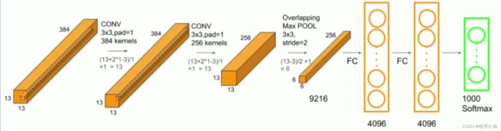
最后得到的特征图的大小为6x6的一个特征图有256个通道
在论文的摘要中提到了:
which has 60 million parameters and 650,000 neurons, consists
of five convolutional layers
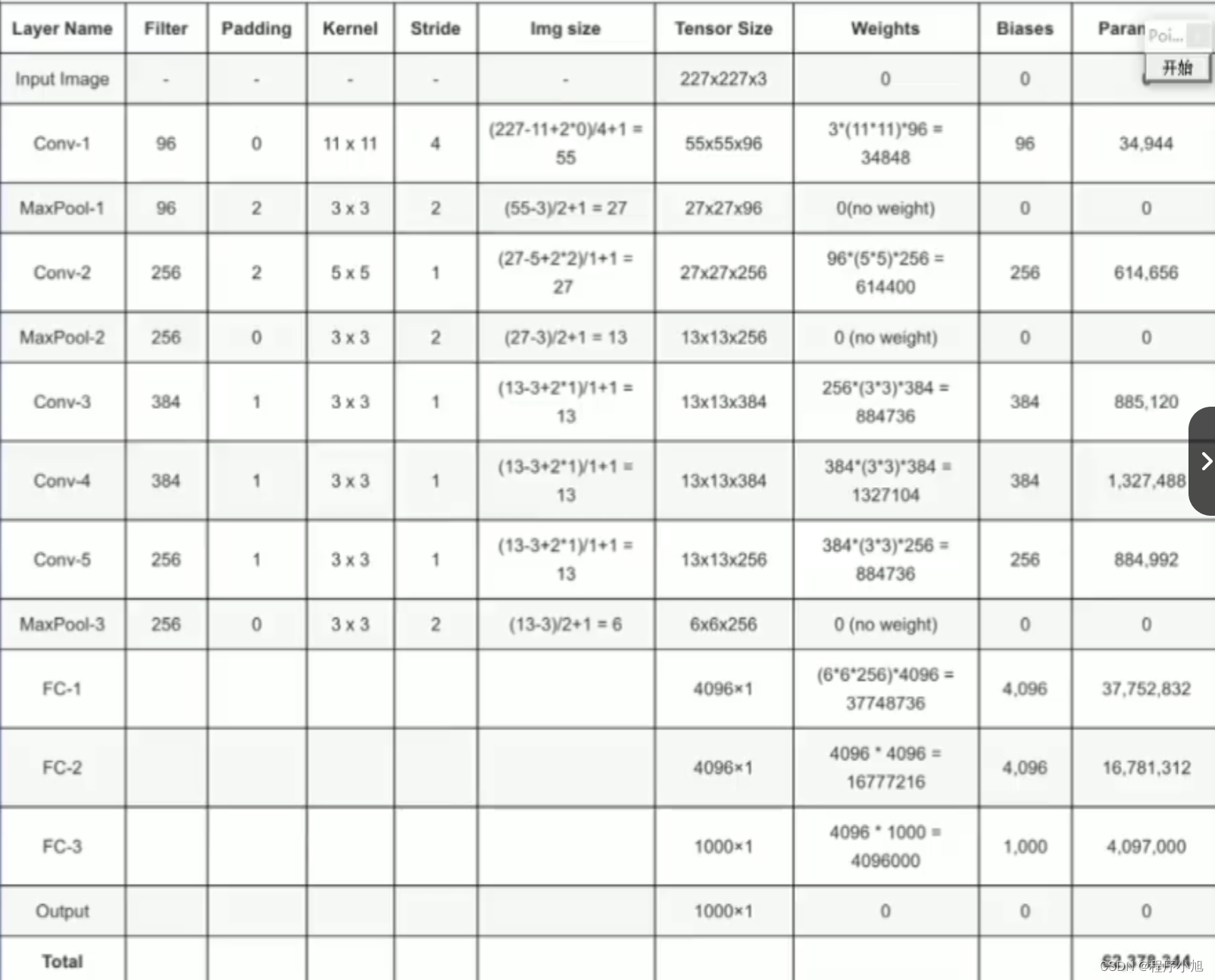
整个alexnet卷积神经网络中含有 60 million个参数,从而引出了参数计算的相关的概念:
F i × ( K s × K s ) × K n + K n F_{i} \times\left(K_{\mathrm{s}} \times K_{\mathrm{s}}\right) \times K_{n}+K_{n} Fi×(Ks×Ks)×Kn+Kn
Fi:输入的通道数
ks:卷积核的尺寸
kh:卷积核的数量(输出的通道数)
结构特点总结
ReLU Nonlinearity
在论文3.1的介绍中使用了relu (3.1 ReLU Nonlinearity)
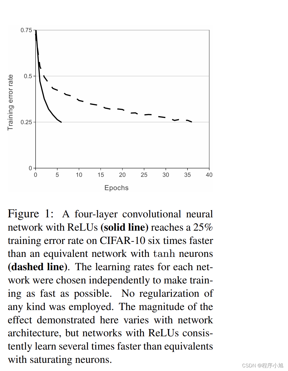
论文中通过4层的卷积网络来训练CIFAR的结果如图所示,虚线表示的是使用双曲正切函数,需要36个批次,而使用relu激活函数,需要10个批次,训练的速度得到显著的提升。
Local Response Normalization
局部响应标准化:有助于AlexNet泛化能力的提升受真实神经元侧抑制(lateralinhibition)启发
侧抑制:细胞分化变为不同时,它会对周围细胞产
生抑制它们向相同方向分化,最终表现为细胞命运的不同
在LRN中论文中提到了一个公式:
b x , y i = a x , y i / ( k + α ∑ j = max ( 0 , i − n / 2 ) min ( N − 1 , i + n / 2 ) ( a x , y j ) 2 ) β b_{x, y}^{i}=a_{x, y}^{i} /\left(k+\alpha \sum_{j=\max (0, i-n / 2)}^{\min (N-1, i+n / 2)}\left(a_{x, y}^{j}\right)^{2}\right)^{\beta} bx,yi=ax,yi/ k+αj=max(0,i−n/2)∑min(N−1,i+n/2)(ax,yj)2 β
Overlapping Pooling(有重叠的池化)
Pooling layers in CNNs summarize the outputs of neighboring groups of neurons in the same kernel map. Traditionally, the neighborhoods summarized by adjacent pooling units do not overlap (e.g.,[17, 11, 4]). To be more precise, a pooling layer can be thought of as consisting of a grid of pooling units spaced s pixels apart, each summarizing a neighborhood of size z × z centered at the location of the pooling unit. If we set s = z, we obtain traditional local pooling as commonly employed
in CNNs. If we set s < z, we obtain overlapping pooling. This is what we use throughout our network, with s = 2 and z = 3. This scheme reduces the top-1 and top-5 error rates by 0.4% and
0.3%, respectively, as compared with the non-overlapping scheme s = 2, z = 2, which produces output of equivalent dimensions. We generally observe during training that models with overlapping pooling find it slightly more difficult to overfit.
根据论文的描述信息:其中s表示的是步长,而z表示的是卷积核
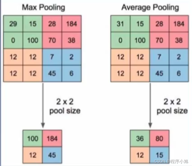
默认移动论文之中所描述的s=z=2的大小,而有重叠的池化本质上就是移动的步长小于卷积核核的大小(s < z)这种情况会出现重叠的区域。
但是可以提高模型的能力。
训练技巧
训练技巧也是论文中的第4部分提到的降低过拟合
Data Augmentation
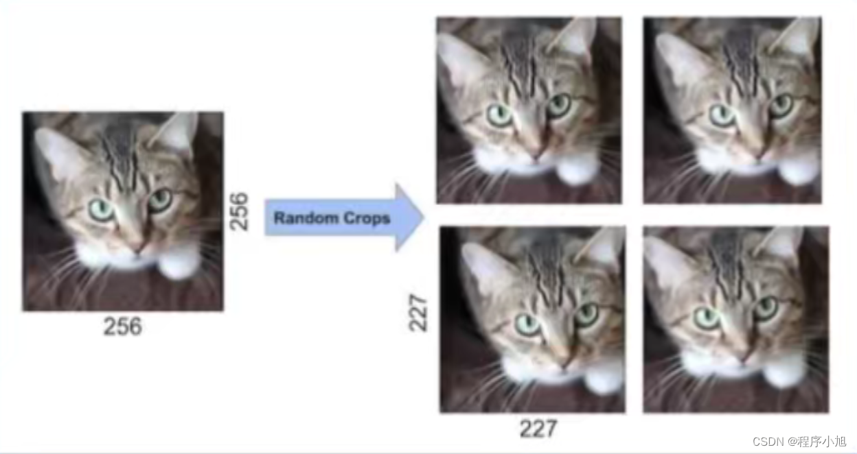
The first form of data augmentation consists of generating image translations and horizontal reflections. We do this by extracting random 224 × 224 patches (and their horizontal reflections) from the
256×256 images and training our network on these extracted patches4
. This increases the size of our
training set by a factor of 2048, though the resulting training examples are, of course, highly interdependent. Without this scheme, our network suffers from substantial overfitting, which would have
forced us to use much smaller networks. At test time, the network makes a prediction by extracting
five 224 × 224 patches (the four corner patches and the center patch) as well as their horizontal
reflections (hence ten patches in all), and averaging the predictions made by the network’s softmax
layer on the ten patches.
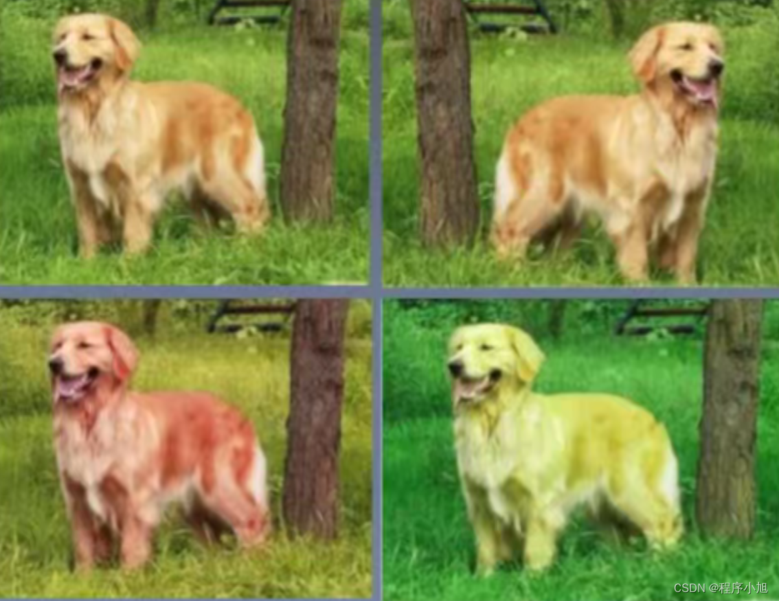
The second form of data augmentation consists of altering the intensities of the RGB channels in
training images. Specifically, we perform PCA on the set of RGB pixel values throughout the
ImageNet training set. To each training image, we add multiples of the found principal components,
第一种数据增强形式包括生成图像平移和水平翻转。为此,我们从256×256图像中随机提取 224×224补丁(及其水平翻转),并在这些提取的补丁上训练我们的网络4。这样,我们的训练集的大小就增加了2048倍,当然,由此产生的训练示例是高度相互依赖的。如果没有这个方案,我们的网络就会出现严重的过拟合问题,这将迫使我们使用更小的网络。
测试时,网络通过提取五个224×224补丁(四个角补丁和中心补丁)及其水平反射(因此总共有十个补丁)来进行预测,并对网络的softmax层在这十个补丁上做出的预测取平均值。
其中2048的计算方法为:256-224=32 32x32=1024 1024x2 =2048
第二种数据增强方式是改变训练图像中RGB通道的强度。具体来说,我们在整个imageNet训练集中的RGB 像素值集合上执行PCA。在每张训练图像中,我们都会添加所发现主成分的倍数
方法一:针对位置
- 训练阶段:
- 图片统一缩放至256*256
- 随机位置裁剪出224*224区域
- 随机进行水平翻转
- 测试阶段
- 图片统—缩放至256*256
- 裁剪出5个224*224区域
- 均进行水平翻转,共得到10张224*224图片
Dropout
随机失活方法,或者叫做暂退法。在该论文中的p=0.5
参考之前的博客,或者动手学深度学习李沐老师的讲解
实验结果及其分析
集成训练
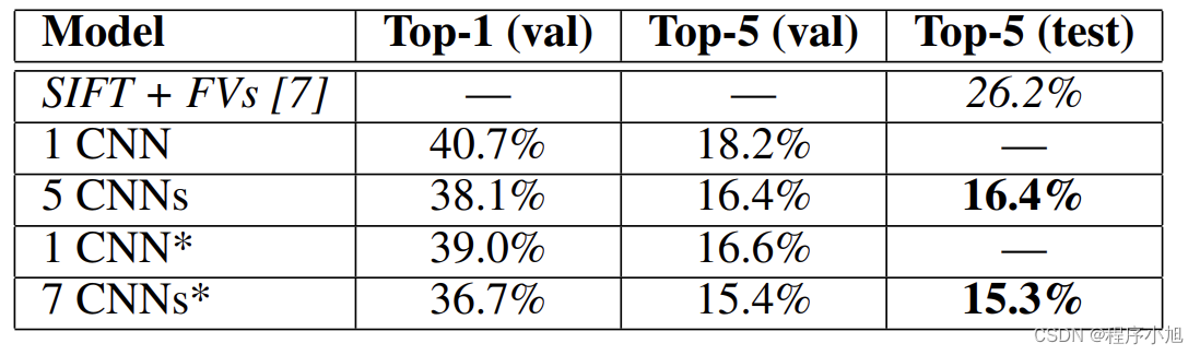
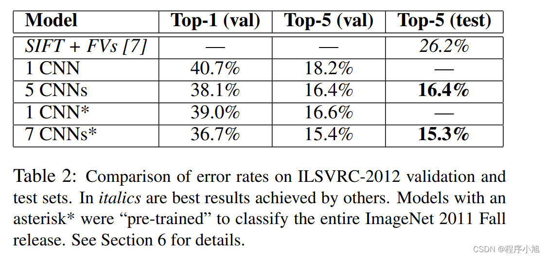
ILSVRC-2012分类指标 :SIFT+FVS:ILSVRC-2012分类任务第二名
- 1CNN:训练一个AlexNet
- 5CNNs:训练五个AlexNet取平均值
- 1CNN*在最后一个池化层之后,额外添加第六个卷积层
并使用lmageNet2011(秋)数据集上预训l练 - 7CNNs*两个预训练微调,与5CNNs取平均值
(集成的思想)
卷积核可视化
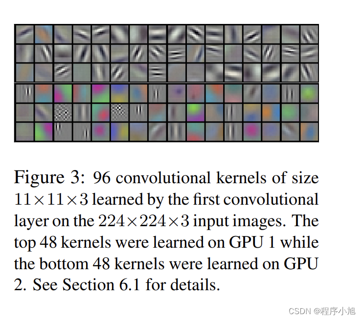
Figure 3 shows the convolutional kernels learned by the network’s two data-connected layers. The
network has learned a variety of frequency- and orientation-selective kernels, as well as various colored blobs. Notice the specialization exhibited by the two GPUs, a result of the restricted connectivity described in Section 3.5. The kernels on GPU 1 are largely color-agnostic, while the kernels
on on GPU 2 are largely color-specific. This kind of specialization occurs during every run and is
independent of any particular random weight initialization (modulo a renumbering of the GPUs)
图3显示了网络的两个数据连接层学习到的卷积核。该网络学习了各种频率和方向选择性 内核,以及各种色块。请注意两个GPU所表现出的专业化,这是第3.5节中描述的受限连接的结果。GPU1上的内核在很大程度上与颜色无关,而GPU2上的内核在很大程度上与颜色有关。这种特殊化在每次运行时都会发生,与任何特定的随机权重初始化无关(GPU
重新编号的修改)。
补充学习卷积的过程在学习一些什么,拓展更为具体的层面上