当前位置：首页 > news >正文

昇思25天学习打卡营第17天|SSD目标检测

news 来源：原创 2024/9/20 3:43:59

学AI还能赢奖品？每天30分钟，25天打通AI任督二脉 (qq.com)

SSD目标检测

模型简介

SSD，全称Single Shot MultiBox Detector，是Wei Liu在ECCV 2016上提出的一种目标检测算法。使用Nvidia Titan X在VOC 2007测试集上，SSD对于输入尺寸300x300的网络，达到74.3%mAP(mean Average Precision)以及59FPS；对于512x512的网络，达到了76.9%mAP ，超越当时最强的Faster RCNN(73.2%mAP)。具体可参考论文[1]。 SSD目标检测主流算法分成可以两个类型：

two-stage方法：RCNN系列

通过算法产生候选框，然后再对这些候选框进行分类和回归。
one-stage方法：YOLO和SSD

直接通过主干网络给出类别位置信息，不需要区域生成。

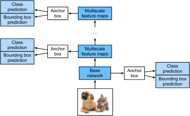
SSD是单阶段的目标检测算法，通过卷积神经网络进行特征提取，取不同的特征层进行检测输出，所以SSD是一种多尺度的检测方法。在需要检测的特征层，直接使用一个3 ×× 3卷积，进行通道的变换。SSD采用了anchor的策略，预设不同长宽比例的anchor，每一个输出特征层基于anchor预测多个检测框（4或者6）。采用了多尺度检测方法，浅层用于检测小目标，深层用于检测大目标。SSD的框架如下图：

SSD-1

模型结构

SSD采用VGG16作为基础模型，然后在VGG16的基础上新增了卷积层来获得更多的特征图以用于检测。SSD的网络结构如图所示。上面是SSD模型，下面是YOLO模型，可以明显看到SSD利用了多尺度的特征图做检测。

SSD-2

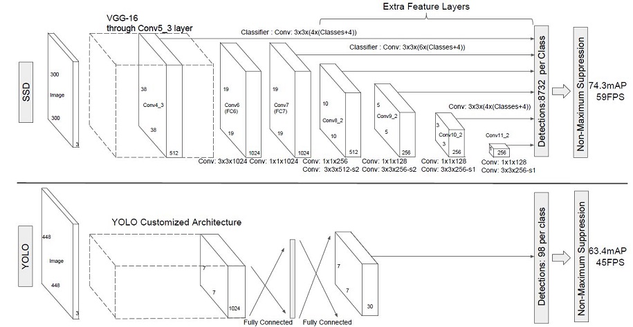
两种单阶段目标检测算法的比较：
SSD先通过卷积不断进行特征提取，在需要检测物体的网络，直接通过一个3 ×× 3卷积得到输出，卷积的通道数由anchor数量和类别数量决定，具体为(anchor数量*(类别数量+4))。
SSD对比了YOLO系列目标检测方法，不同的是SSD通过卷积得到最后的边界框，而YOLO对最后的输出采用全连接的形式得到一维向量，对向量进行拆解得到最终的检测框。

模型特点

多尺度检测

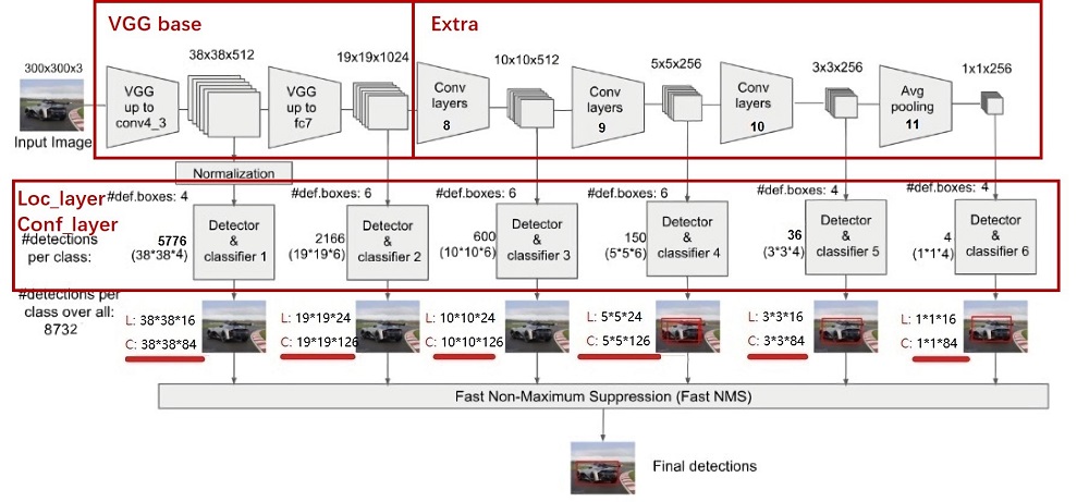
在SSD的网络结构图中我们可以看到，SSD使用了多个特征层，特征层的尺寸分别是38 ×× 38，19 ×× 19，10 ×× 10，5 ×× 5，3 ×× 3，1 ×× 1，一共6种不同的特征图尺寸。大尺度特征图（较靠前的特征图）可以用来检测小物体，而小尺度特征图（较靠后的特征图）用来检测大物体。多尺度检测的方式，可以使得检测更加充分（SSD属于密集检测），更能检测出小目标。
采用卷积进行检测

与YOLO最后采用全连接层不同，SSD直接采用卷积对不同的特征图来进行提取检测结果。对于形状为m ×× n ×× p的特征图，只需要采用3 ×× 3 ×× p这样比较小的卷积核得到检测值。
预设anchor

在YOLOv1中，直接由网络预测目标的尺寸，这种方式使得预测框的长宽比和尺寸没有限制，难以训练。在SSD中，采用预设边界框，我们习惯称它为anchor（在SSD论文中叫default bounding boxes），预测框的尺寸在anchor的指导下进行微调。

环境准备

本案例基于MindSpore实现，开始实验前，请确保本地已经安装了mindspore、download、pycocotools、opencv-python。

%%capture captured_output
# 实验环境已经预装了mindspore==2.2.14，如需更换mindspore版本，可更改下面mindspore的版本号
!pip uninstall mindspore -y
!pip install -i https://pypi.mirrors.ustc.edu.cn/simple mindspore==2.2.14

# 查看当前 mindspore 版本
!pip show mindspore

Name: mindspore
Version: 2.2.14
Summary: MindSpore is a new open source deep learning training/inference framework that could be used for mobile, edge and cloud scenarios.
Home-page: https://www.mindspore.cn
Author: The MindSpore Authors
Author-email: contact@mindspore.cn
License: Apache 2.0
Location: /home/nginx/miniconda/envs/jupyter/lib/python3.9/site-packages
Requires: asttokens, astunparse, numpy, packaging, pillow, protobuf, psutil, scipy
Required-by:

!pip install -i https://pypi.mirrors.ustc.edu.cn/simple pycocotools==2.0.7

Looking in indexes: https://pypi.mirrors.ustc.edu.cn/simple
Collecting pycocotools==2.0.7Downloading https://mirrors.bfsu.edu.cn/pypi/web/packages/19/93/5aaec888e3aa4d05b3a1472f331b83f7dc684d9a6b2645709d8f3352ba00/pycocotools-2.0.7-cp39-cp39-manylinux_2_17_aarch64.manylinux2014_aarch64.whl (419 kB)━━━━━━━━━━━━━━━━━━━━━━━━━━━━━━━━━━━━━━ 419.9/419.9 kB 14.8 MB/s eta 0:00:00
Requirement already satisfied: matplotlib>=2.1.0 in /home/nginx/miniconda/envs/jupyter/lib/python3.9/site-packages (from pycocotools==2.0.7) (3.9.0)
Requirement already satisfied: numpy in /home/nginx/miniconda/envs/jupyter/lib/python3.9/site-packages (from pycocotools==2.0.7) (1.26.4)
Requirement already satisfied: contourpy>=1.0.1 in /home/nginx/miniconda/envs/jupyter/lib/python3.9/site-packages (from matplotlib>=2.1.0->pycocotools==2.0.7) (1.2.1)
Requirement already satisfied: cycler>=0.10 in /home/nginx/miniconda/envs/jupyter/lib/python3.9/site-packages (from matplotlib>=2.1.0->pycocotools==2.0.7) (0.12.1)
Requirement already satisfied: fonttools>=4.22.0 in /home/nginx/miniconda/envs/jupyter/lib/python3.9/site-packages (from matplotlib>=2.1.0->pycocotools==2.0.7) (4.53.0)
Requirement already satisfied: kiwisolver>=1.3.1 in /home/nginx/miniconda/envs/jupyter/lib/python3.9/site-packages (from matplotlib>=2.1.0->pycocotools==2.0.7) (1.4.5)
Requirement already satisfied: packaging>=20.0 in /home/nginx/miniconda/envs/jupyter/lib/python3.9/site-packages (from matplotlib>=2.1.0->pycocotools==2.0.7) (23.2)
Requirement already satisfied: pillow>=8 in /home/nginx/miniconda/envs/jupyter/lib/python3.9/site-packages (from matplotlib>=2.1.0->pycocotools==2.0.7) (10.3.0)
Requirement already satisfied: pyparsing>=2.3.1 in /home/nginx/miniconda/envs/jupyter/lib/python3.9/site-packages (from matplotlib>=2.1.0->pycocotools==2.0.7) (3.1.2)
Requirement already satisfied: python-dateutil>=2.7 in /home/nginx/miniconda/envs/jupyter/lib/python3.9/site-packages (from matplotlib>=2.1.0->pycocotools==2.0.7) (2.9.0.post0)
Requirement already satisfied: importlib-resources>=3.2.0 in /home/nginx/miniconda/envs/jupyter/lib/python3.9/site-packages (from matplotlib>=2.1.0->pycocotools==2.0.7) (6.4.0)
Requirement already satisfied: zipp>=3.1.0 in /home/nginx/miniconda/envs/jupyter/lib/python3.9/site-packages (from importlib-resources>=3.2.0->matplotlib>=2.1.0->pycocotools==2.0.7) (3.17.0)
Requirement already satisfied: six>=1.5 in /home/nginx/miniconda/envs/jupyter/lib/python3.9/site-packages (from python-dateutil>=2.7->matplotlib>=2.1.0->pycocotools==2.0.7) (1.16.0)
Installing collected packages: pycocotools
Successfully installed pycocotools-2.0.7[notice] A new release of pip is available: 24.1 -> 24.1.1
[notice] To update, run: python -m pip install --upgrade pip

数据准备与处理

本案例所使用的数据集为COCO 2017。为了更加方便地保存和加载数据，本案例中在数据读取前首先将COCO数据集转换成MindRecord格式。使用MindSpore Record数据格式可以减少磁盘IO、网络IO开销，从而获得更好的使用体验和性能提升。首先我们需要下载处理好的MindRecord格式的COCO数据集。运行以下代码将数据集下载并解压到指定路径。

from download import downloaddataset_url = "https://mindspore-website.obs.cn-north-4.myhuaweicloud.com/notebook/datasets/ssd_datasets.zip"
path = "./"
path = download(dataset_url, path, kind="zip", replace=True)

Downloading data from https://mindspore-website.obs.cn-north-4.myhuaweicloud.com/notebook/datasets/ssd_datasets.zip (16.0 MB)file_sizes: 100%|███████████████████████████| 16.8M/16.8M [00:00<00:00, 105MB/s]
Extracting zip file...
Successfully downloaded / unzipped to ./

查看MindRecord格式的数据集有哪些列（columns）：

show_mindrecord_file = "./datasets/MindRecord_COCO/ssd_eval.mindrecord0"
show_dataset = MindDataset(show_mindrecord_file)
columns_list = show_dataset.get_col_names()
print("Columns in the MindRecord dataset:", columns_list)

Columns in the MindRecord dataset: ['annotation', 'image', 'img_id']

然后我们为数据处理定义一些输入：

coco_root = "./datasets/"
anno_json = "./datasets/annotations/instances_val2017.json"train_cls = ['background', 'person', 'bicycle', 'car', 'motorcycle', 'airplane', 'bus','train', 'truck', 'boat', 'traffic light', 'fire hydrant','stop sign', 'parking meter', 'bench', 'bird', 'cat', 'dog','horse', 'sheep', 'cow', 'elephant', 'bear', 'zebra','giraffe', 'backpack', 'umbrella', 'handbag', 'tie','suitcase', 'frisbee', 'skis', 'snowboard', 'sports ball','kite', 'baseball bat', 'baseball glove', 'skateboard','surfboard', 'tennis racket', 'bottle', 'wine glass', 'cup','fork', 'knife', 'spoon', 'bowl', 'banana', 'apple','sandwich', 'orange', 'broccoli', 'carrot', 'hot dog', 'pizza','donut', 'cake', 'chair', 'couch', 'potted plant', 'bed','dining table', 'toilet', 'tv', 'laptop', 'mouse', 'remote','keyboard', 'cell phone', 'microwave', 'oven', 'toaster', 'sink','refrigerator', 'book', 'clock', 'vase', 'scissors','teddy bear', 'hair drier', 'toothbrush']train_cls_dict = {}
for i, cls in enumerate(train_cls):train_cls_dict[cls] = i

打开terminal查看下载的目录结构和大小：

[nginx@cloud-5e09579c-3e80-4044-9884-9fa9e43986ea-c5d5d8448-pdzs5 datasets]$ ls -R .
.:
MindRecord_COCO  annotations  train2017  val2017./MindRecord_COCO:
ssd.mindrecord0  ssd.mindrecord0.db  ssd.mindrecord1  ssd.mindrecord1.db  ssd_eval.mindrecord0  ssd_eval.mindrecord0.db  ssd_eval.mindrecord1  ssd_eval.mindrecord1.db./annotations:
instances_train2017.json  instances_val2017.json./train2017:
000000005802.jpg  000000079841.jpg  000000144941.jpg  000000193271.jpg  000000242611.jpg  000000309022.jpg  000000360772.jpg  000000384553.jpg  000000462565.jpg  000000542145.jpg
000000012448.jpg  000000086408.jpg  000000166532.jpg  000000204805.jpg  000000262284.jpg  000000318219.jpg  000000368402.jpg  000000386164.jpg  000000483108.jpg  000000554625.jpg
000000051191.jpg  000000111076.jpg  000000173350.jpg  000000222564.jpg  000000269105.jpg  000000324266.jpg  000000372938.jpg  000000391895.jpg  000000515289.jpg  000000562150.jpg
000000060623.jpg  000000113588.jpg  000000184613.jpg  000000223648.jpg  000000293802.jpg  000000328757.jpg  000000374628.jpg  000000403013.jpg  000000522418.jpg  000000574769.jpg
000000060760.jpg  000000118113.jpg  000000191381.jpg  000000224736.jpg  000000294832.jpg  000000337264.jpg  000000384213.jpg  000000412151.jpg  000000540186.jpg  000000579003.jpg./val2017:
000000006818.jpg  000000037777.jpg  000000087038.jpg  000000174482.jpg  000000252219.jpg  000000331352.jpg  000000397133.jpg  000000403385.jpg  000000458054.jpg  000000480985.jpg
[nginx@cloud-5e09579c-3e80-4044-9884-9fa9e43986ea-c5d5d8448-pdzs5 datasets]$ du -sh
202M    .

查看其中一个图片：

import os
import matplotlib.pyplot as plt
from PIL import Image# 设置数据集路径
dataset_path = "datasets/train2017"# 获取数据集中的所有图像文件名
image_files = os.listdir(dataset_path)# 选择一个图像文件进行显示
image_file = image_files[0]
image_path = os.path.join(dataset_path, image_file)# 打开并显示图像
image = Image.open(image_path)
plt.imshow(image)
plt.show()

查看标注文件：

import json# 打开训练集标注文件并打印内容
with open('datasets/annotations/instances_train2017.json', 'r') as file:train_data = json.load(file)print("Training Data:")print(json.dumps(train_data, indent=4))# 打开验证集标注文件并打印内容
with open('datasets/annotations/instances_val2017.json', 'r') as file:val_data = json.load(file)print("Validation Data:")print(json.dumps(val_data, indent=4))

Training Data:
{
"images": [
{
"license": 3,
"file_name": "000000391895.jpg",
"coco_url": "http://images.cocodataset.org/train2017/000000391895.jpg",
"height": 360,
"width": 640,
"date_captured": "2013-11-14 11:18:45",
"flickr_url": "http://farm9.staticflickr.com/8186/8119368305_4e622c8349_z.jpg",
"id": 391895
},
{
"license": 4,
"file_name": "000000522418.jpg",
"coco_url": "http://images.cocodataset.org/train2017/000000522418.jpg",
"height": 480,
"width": 640,
"date_captured": "2013-11-14 11:38:44",
"flickr_url": "http://farm1.staticflickr.com/1/127244861_ab0c0381e7_z.jpg",
"id": 522418
},
。。。。。。

"annotations": [
{
"segmentation": [
[
376.97,
176.91,
398.81,
176.91,
396.38,
147.78,
447.35,
146.17,
448.16,
172.05,
448.16,
178.53,
464.34,
186.62,
464.34,
192.28,
448.97,
195.51,
447.35,
235.96,
441.69,
258.62,
454.63,
268.32,
462.72,
276.41,
471.62,
290.98,
456.25,
298.26,
439.26,
292.59,
431.98,
308.77,
442.49,
313.63,
436.02,
316.86,
429.55,
322.53,
419.84,
354.89,
402.04,
359.74,
401.24,
312.82,
370.49,
303.92,
391.53,
299.87,
391.53,
280.46,
385.06,
278.84,
381.01,
278.84,
359.17,
269.13,
373.73,
261.85,
374.54,
256.19,
378.58,
231.11,
383.44,
205.22,
385.87,
192.28,
373.73,
184.19
]
],
"area": 12190.44565,
"iscrowd": 0,
"image_id": 391895,
"bbox": [
359.17,
146.17,
112.45,
213.57
],
"category_id": 4,
"id": 151091
},
{
"segmentation": [
[
352.55,
146.82,
353.61,
137.66,
356.07,
112.66,
357.13,
94.7,
357.13,
84.49,
363.12,
73.92,
370.16,
68.64,
370.16,
66.53,
368.4,
63.71,
368.05,
54.56,
361.0,
53.85,
356.07,
50.33,
356.43,
46.46,
364.17,
42.23,
369.1,
35.89,
371.22,
30.96,
376.85,
26.39,
383.54,
22.16,
391.29,
23.22,
400.79,
27.79,
402.2,
30.61,
404.32,
34.84,
406.08,
38.71,
406.08,
41.53,
406.08,
47.87,
407.84,
54.91,
408.89,
59.84,
408.89,
61.25,
408.89,
63.36,
422.28,
67.94,
432.13,
72.52,
445.87,
81.32,
446.57,
84.14,
446.57,
99.2,
451.15,
118.22,
453.26,
128.39,
453.61,
131.92,
453.61,
133.68,
451.5,
137.55,
451.5,
139.31,
455.38,
144.24,
455.38,
153.04,
455.73,
155.16,
461.01,
162.85,
462.07,
166.37,
459.95,
170.6,
459.6,
176.58,
459.95,
178.69,
459.95,
180.1,
448.33,
180.45,
447.98,
177.64,
446.57,
172.36,
447.63,
166.37,
449.74,
160.38,
450.09,
157.57,
448.68,
152.28,
445.16,
147.71,
441.29,
143.48,
435.66,
142.78,
428.26,
141.37,
420.87,
141.37,
418.75,
141.37,
411.71,
144.19,
404.32,
145.24,
396.57,
150.52,
395.87,
152.64,
391.29,
157.92,
391.99,
164.26,
389.53,
172.0,
389.53,
176.23,
376.85,
174.82,
375.09,
177.29,
374.03,
188.55,
381.08,
192.78,
384.6,
194.19,
384.95,
198.41,
383.19,
203.34,
380.02,
210.03,
378.61,
218.84,
375.79,
220.95,
373.68,
223.42,
368.05,
245.56,
368.05,
256.48,
368.05,
259.3,
360.65,
261.06,
361.71,
266.34,
361.36,
268.8,
358.19,
271.62,
353.26,
274.09,
349.74,
275.49,
341.28,
273.03,
339.88,
270.21,
343.05,
263.52,
347.62,
259.65,
351.5,
253.31,
352.9,
250.84,
356.07,
244.86,
359.24,
235.35,
357.83,
214.58,
357.13,
204.36,
358.89,
196.97,
361.71,
183.94,
365.93,
175.14,
371.92,
169.15,
376.15,
164.22,
377.2,
160.35,
378.61,
151.9,
377.55,
145.56,
375.79,
131.82,
375.09,
131.82,
373.33,
139.22,
370.16,
143.8,
369.1,
148.02,
365.93,
155.42,
361.0,
158.59,
358.89,
159.99,
358.89,
161.76,
361.71,
163.87,
363.12,
165.98,
363.12,
168.8,
362.06,
170.21,
360.3,
170.56,
358.54,
170.56,
355.02,
168.45,
352.2,
163.52,
351.14,
161.05,
351.14,
156.83,
352.2,
154.36,
353.26,
152.25,
353.61,
152.25,
353.26,
149.43
],
[
450.45,
196.54,
461.71,
195.13,
466.29,
209.22,
469.11,
227.88,
475.09,
241.62,
479.32,
249.01,
482.49,
262.04,
482.84,
279.96,
485.66,
303.87,
492.7,
307.04,
493.76,
309.5,
491.29,
318.66,
490.59,
321.83,
485.66,
322.89,
480.02,
322.89,
475.45,
317.96,
474.74,
310.91,
470.87,
304.57,
470.87,
294.71,
467.7,
282.34,
463.47,
276.7,
461.71,
272.83,
459.25,
270.01,
454.32,
268.25,
450.09,
259.82,
450.09,
252.07,
445.52,
234.11,
449.04,
229.57,
448.33,
199.29
]
],
"area": 14107.271300000002,
"iscrowd": 0,
"image_id": 391895,
"bbox": [
339.88,
22.16,
153.88,
300.73
],
"category_id": 1,
"id": 202758
},
。。。。。。

"categories": [
{
"supercategory": "person",
"id": 1,
"name": "person"
},
{
"supercategory": "vehicle",
"id": 2,
"name": "bicycle"
},
。。。。。。

"type": "instances",
"info": {
"description": "This is stable 1.0 version of the 2014 MS COCO dataset.",
"url": "http:\\/\\/mscoco.org",
"version": "1.0",
"year": 2014,
"contributor": "Microsoft COCO group",
"date_created": "2015-01-27 09:11:52.357475"
},
"licenses": [
{
"url": "http:\\/\\/creativecommons.org\\/licenses\\/by-nc-sa\\/2.0\\/",
"id": 1,
"name": "Attribution-NonCommercial-ShareAlike License"
},
{
"url": "http:\\/\\/creativecommons.org\\/licenses\\/by-nc\\/2.0\\/",
"id": 2,
"name": "Attribution-NonCommercial License"
},
。。。。。。
Validation Data:

。。。。。。

"categories"是一个包含类别信息的列表。每个类别都有一个唯一的ID和一个名称。这些类别通常对应于图像中的对象或实体，例如人、汽车、动物等。

每个类别的信息包括：

"id": 类别的唯一标识符，通常是整数。
"name": 类别的名称，例如"person"、"car"、"dog"等。
"supercategory": 可选字段，表示该类别所属的大类，例如"animal"、"vehicle"等。

在COCO数据集的标注文件中，"segmentation"是一个包含分割信息的字段。它用于描述图像中对象或实体的边界框（bounding box）和分割区域（segmentation area）。这里是使用的边界框（bounding box）。

例如：

第一个多边形的顶点坐标列表：

[352.55, 146.82, 353.61, 137.66, 356.07, 112.66, 357.13, 94.7, 357.13, 84.49, 363.12, 73.92, 370.16, 68.64, 370.16, 66.53, 368.4, 63.71, 368.05, 54.56, 361.0, 53.85, 356.07, 50.33, 356.43, 46.46, 364.17, 42.23, 369.1, 35.89, 371.22, 30.96, 376.85, 26.39, 383.54, 22.16, 391.29, 23.22, 400.79, 27.79, 402.2, 30.61, 404.32, 34.84, 406.08, 38.71, 406.08, 41.53, 406.08, 47.87, 407.84, 54.91, 408.89, 59.84, 408.89, 61.25, 408.89, 63.36, 422.28, 67.94, 432.13, 72.52, 445.87, 81.32, 446.57, 84.14, 446.57, 99.2, 451.15, 118.22, 453.26, 128.39, 453.61, 131.92, 453.61, 133.68, 451.5, 137.55, 451.5, 139.31, 455.38, 144.24, 455.38, 153.04, 455.73, 155.16, 461.01, 162.85, 462.07, 166.37, 459.95, 170.6, 459.6, 176.58, 459.95, 178.69, 459.95, 180.1, 448.33, 180.45, 447.98, 177.64, 446.57, 172.36, 447.63, 166.37, 449.74, 160.38, 450.09, 157.57, 448.68, 152.28, 445.16, 147.71, 441.29, 143.48, 435.66, 142.78, 428.26, 141.37, 420.87, 141.37, 418.75, 141.37, 411.71, 144.19, 404.32, 145.24, 396.57, 150.52, 395.87, 152.64, 391.29, 157.92, 391.99, 164.26, 389.53, 172.0, 389.53, 176.23, 376.85, 174.82, 375.09, 177.29, 374.03, 188.55, 381.08, 192.78, 384.6, 194.19, 384.95, 198.41, 383.19, 203.34, 380.02, 210.03, 378.61, 218.84, 375.79, 220.95, 373.68, 223.42, 368.05, 245.56, 368.05, 256.48, 368.05, 259.3, 360.65, 261.06, 361.71, 266.34, 361.36, 268.8, 358.19, 271.62, 353.26, 274.09, 349.74, 275.49, 341.28, 273.03, 339.88, 270.21, 343.05, 263.52, 347.62, 259.65, 351.5, 253.31, 352.9, 250.84, 356.07, 244.86, 359.24, 235.35, 357.83, 214.58, 357.13, 204.36, 358.89, 196.97, 361.71, 183.94, 365.93, 175.14, 371.92, 169.15, 376.15, 164.22, 377.2, 160.35, 378.61, 151.9, 377.55, 145.56, 375.79, 131.82, 375.09, 131.82, 373.33, 139.22, 370.16, 143.8, 369.1, 148.02, 365.93, 155.42, 361.0, 158.59, 358.89, 159.99, 358.89, 161.76, 361.71, 163.87, 363.12, 165.98, 363.12, 168.8, 362.06, 170.21, 360.3, 170.56, 358.54, 170.56, 355.02, 168.45, 352.2, 163.52, 351.14, 161.05, 351.14, 156.83, 352.2, 154.36, 353.26, 152.25, 353.61, 152.25, 353.26, 149.43
]

第二个多边形的顶点坐标列表：

[450.45, 196.54, 461.71, 195.13, 466.29, 209.22, 469.11, 227.88, 475.09, 241.62, 479.32, 249.01, 482.49, 262.04, 482.84, 279.96, 485.66, 303.87, 492.7, 307.04, 493.76, 309.5, 491.29, 318.66, 490.59, 321.83, 485.66, 322.89, 480.02, 322.89, 475.45, 317.96, 474.74, 310.91, 470.87, 304.57, 470.87, 294.71, 467.7, 282.34, 463.47, 276.7, 461.71, 272.83, 459.25, 270.01, 454.32, 268.25, 450.09, 259.82, 450.09, 252.07, 445.52, 234.11, 449.04, 229.57, 448.33, 199.29
]

其他字段的含义如下：

"area": 对象的面积，单位是像素。
"iscrowd": 表示对象是否是拥挤的（通常用于处理多个对象紧密相连的情况）。
"image_id": 图像的唯一标识符。
"bbox": 对象的边界框，格式为 [x, y, width, height]，表示左上角坐标和框的宽度和高度。
"category_id": 对象的类别标识符。
"id": 标注的唯一标识符。

打印类别、边界框：

import json# 读取训练集标注文件
with open("datasets/annotations/instances_train2017.json", "r") as f:train_annotations = json.load(f)# 读取验证集标注文件
with open("datasets/annotations/instances_val2017.json", "r") as f:val_annotations = json.load(f)# 打印训练集前5个标注信息的类别和边界框
for i in range(5):print("Train image {}:".format(i))print("Category: {}".format(train_annotations["annotations"][i]["category_id"]))print("Bounding box: {}".format(train_annotations["annotations"][i]["bbox"]))print()# 打印验证集前5个标注信息的类别和边界框
for i in range(5):print("Validation image {}:".format(i))print("Category: {}".format(val_annotations["annotations"][i]["category_id"]))print("Bounding box: {}".format(val_annotations["annotations"][i]["bbox"]))print()

Train image 0:
Category: 4
Bounding box: [359.17, 146.17, 112.45, 213.57]Train image 1:
Category: 1
Bounding box: [339.88, 22.16, 153.88, 300.73]Train image 2:
Category: 1
Bounding box: [471.64, 172.82, 35.92, 48.1]Train image 3:
Category: 2
Bounding box: [486.01, 183.31, 30.63, 34.98]Train image 4:
Category: 1
Bounding box: [382.48, 0.0, 256.8, 474.31]Validation image 0:
Category: 44
Bounding box: [217.62, 240.54, 38.99, 57.75]Validation image 1:
Category: 67
Bounding box: [1.0, 240.24, 346.63, 186.76]Validation image 2:
Category: 1
Bounding box: [388.66, 69.92, 109.41, 277.62]Validation image 3:
Category: 49
Bounding box: [135.57, 249.43, 22.32, 28.79]Validation image 4:
Category: 51
Bounding box: [31.28, 344.0, 68.12, 40.83]

COCO 2017数据集是一个大规模的图像识别、分割和字幕任务的数据集，广泛应用于计算机视觉研究和模型训练。

COCO 2017数据集的全称是Common Objects in Context，由微软团队提供支持，主要用于图像识别。这个数据集包含train（118,287张）、val（5,000张）和test（40,670张）三个部分。这些图像涵盖了80个不同的目标类别和91种材料类别，总共有150万个目标实例。每张图像还附带有五句描述性语句。这使得COCO 2017数据集不仅适用于对象检测，还适用于语义分割、实例分割、图像标题生成等多种任务。

该数据集以JSON格式存储，包含图像信息、注释信息、类别信息等。每个注释文件不仅包含图像的文件名和尺寸，还详细记录了对象的边界框坐标、分割掩模以及关键点等信息。这些丰富的信息为各种计算机视觉任务提供了强有力的支持。例如，在对象检测任务中，可以通过这些边界框来定位和分类图像中的各种目标。

数据采样

为了使模型对于各种输入对象大小和形状更加鲁棒，SSD算法每个训练图像通过以下选项之一随机采样：

使用整个原始输入图像
采样一个区域，使采样区域和原始图片最小的交并比重叠为0.1,0.3,0.5,0.7或0.9
随机采样一个区域

每个采样区域的大小为原始图像大小的[0.3,1]，长宽比在1/2和2之间。如果真实标签框中心在采样区域内，则保留两者重叠部分作为新图片的真实标注框。在上述采样步骤之后，将每个采样区域大小调整为固定大小，并以0.5的概率水平翻转。

import cv2
import numpy as npdef _rand(a=0., b=1.):return np.random.rand() * (b - a) + adef intersect(box_a, box_b):"""Compute the intersect of two sets of boxes."""max_yx = np.minimum(box_a[:, 2:4], box_b[2:4])min_yx = np.maximum(box_a[:, :2], box_b[:2])inter = np.clip((max_yx - min_yx), a_min=0, a_max=np.inf)return inter[:, 0] * inter[:, 1]def jaccard_numpy(box_a, box_b):"""Compute the jaccard overlap of two sets of boxes."""inter = intersect(box_a, box_b)area_a = ((box_a[:, 2] - box_a[:, 0]) *(box_a[:, 3] - box_a[:, 1]))area_b = ((box_b[2] - box_b[0]) *(box_b[3] - box_b[1]))union = area_a + area_b - interreturn inter / uniondef random_sample_crop(image, boxes):"""Crop images and boxes randomly."""height, width, _ = image.shapemin_iou = np.random.choice([None, 0.1, 0.3, 0.5, 0.7, 0.9])if min_iou is None:return image, boxesfor _ in range(50):image_t = imagew = _rand(0.3, 1.0) * widthh = _rand(0.3, 1.0) * height# aspect ratio constraint b/t .5 & 2if h / w < 0.5 or h / w > 2:continueleft = _rand() * (width - w)top = _rand() * (height - h)rect = np.array([int(top), int(left), int(top + h), int(left + w)])overlap = jaccard_numpy(boxes, rect)# dropout some boxesdrop_mask = overlap > 0if not drop_mask.any():continueif overlap[drop_mask].min() < min_iou and overlap[drop_mask].max() > (min_iou + 0.2):continueimage_t = image_t[rect[0]:rect[2], rect[1]:rect[3], :]centers = (boxes[:, :2] + boxes[:, 2:4]) / 2.0m1 = (rect[0] < centers[:, 0]) * (rect[1] < centers[:, 1])m2 = (rect[2] > centers[:, 0]) * (rect[3] > centers[:, 1])# mask in that both m1 and m2 are truemask = m1 * m2 * drop_mask# have any valid boxes? try again if notif not mask.any():continue# take only matching gt boxesboxes_t = boxes[mask, :].copy()boxes_t[:, :2] = np.maximum(boxes_t[:, :2], rect[:2])boxes_t[:, :2] -= rect[:2]boxes_t[:, 2:4] = np.minimum(boxes_t[:, 2:4], rect[2:4])boxes_t[:, 2:4] -= rect[:2]return image_t, boxes_treturn image, boxesdef ssd_bboxes_encode(boxes):"""Labels anchors with ground truth inputs."""def jaccard_with_anchors(bbox):"""Compute jaccard score a box and the anchors."""# Intersection bbox and volume.ymin = np.maximum(y1, bbox[0])xmin = np.maximum(x1, bbox[1])ymax = np.minimum(y2, bbox[2])xmax = np.minimum(x2, bbox[3])w = np.maximum(xmax - xmin, 0.)h = np.maximum(ymax - ymin, 0.)# Volumes.inter_vol = h * wunion_vol = vol_anchors + (bbox[2] - bbox[0]) * (bbox[3] - bbox[1]) - inter_voljaccard = inter_vol / union_volreturn np.squeeze(jaccard)pre_scores = np.zeros((8732), dtype=np.float32)t_boxes = np.zeros((8732, 4), dtype=np.float32)t_label = np.zeros((8732), dtype=np.int64)for bbox in boxes:label = int(bbox[4])scores = jaccard_with_anchors(bbox)idx = np.argmax(scores)scores[idx] = 2.0mask = (scores > matching_threshold)mask = mask & (scores > pre_scores)pre_scores = np.maximum(pre_scores, scores * mask)t_label = mask * label + (1 - mask) * t_labelfor i in range(4):t_boxes[:, i] = mask * bbox[i] + (1 - mask) * t_boxes[:, i]index = np.nonzero(t_label)# Transform to tlbr.bboxes = np.zeros((8732, 4), dtype=np.float32)bboxes[:, [0, 1]] = (t_boxes[:, [0, 1]] + t_boxes[:, [2, 3]]) / 2bboxes[:, [2, 3]] = t_boxes[:, [2, 3]] - t_boxes[:, [0, 1]]# Encode features.bboxes_t = bboxes[index]default_boxes_t = default_boxes[index]bboxes_t[:, :2] = (bboxes_t[:, :2] - default_boxes_t[:, :2]) / (default_boxes_t[:, 2:] * 0.1)tmp = np.maximum(bboxes_t[:, 2:4] / default_boxes_t[:, 2:4], 0.000001)bboxes_t[:, 2:4] = np.log(tmp) / 0.2bboxes[index] = bboxes_tnum_match = np.array([len(np.nonzero(t_label)[0])], dtype=np.int32)return bboxes, t_label.astype(np.int32), num_matchdef preprocess_fn(img_id, image, box, is_training):"""Preprocess function for dataset."""cv2.setNumThreads(2)def _infer_data(image, input_shape):img_h, img_w, _ = image.shapeinput_h, input_w = input_shapeimage = cv2.resize(image, (input_w, input_h))# When the channels of image is 1if len(image.shape) == 2:image = np.expand_dims(image, axis=-1)image = np.concatenate([image, image, image], axis=-1)return img_id, image, np.array((img_h, img_w), np.float32)def _data_aug(image, box, is_training, image_size=(300, 300)):ih, iw, _ = image.shapeh, w = image_sizeif not is_training:return _infer_data(image, image_size)# Random cropbox = box.astype(np.float32)image, box = random_sample_crop(image, box)ih, iw, _ = image.shape# Resize imageimage = cv2.resize(image, (w, h))# Flip image or notflip = _rand() < .5if flip:image = cv2.flip(image, 1, dst=None)# When the channels of image is 1if len(image.shape) == 2:image = np.expand_dims(image, axis=-1)image = np.concatenate([image, image, image], axis=-1)box[:, [0, 2]] = box[:, [0, 2]] / ihbox[:, [1, 3]] = box[:, [1, 3]] / iwif flip:box[:, [1, 3]] = 1 - box[:, [3, 1]]box, label, num_match = ssd_bboxes_encode(box)return image, box, label, num_matchreturn _data_aug(image, box, is_training, image_size=[300, 300])

数据集创建

from mindspore import Tensor
from mindspore.dataset import MindDataset
from mindspore.dataset.vision import Decode, HWC2CHW, Normalize, RandomColorAdjustdef create_ssd_dataset(mindrecord_file, batch_size=32, device_num=1, rank=0,is_training=True, num_parallel_workers=1, use_multiprocessing=True):"""Create SSD dataset with MindDataset."""dataset = MindDataset(mindrecord_file, columns_list=["img_id", "image", "annotation"], num_shards=device_num,shard_id=rank, num_parallel_workers=num_parallel_workers, shuffle=is_training)decode = Decode()dataset = dataset.map(operations=decode, input_columns=["image"])change_swap_op = HWC2CHW()# Computed from random subset of ImageNet training imagesnormalize_op = Normalize(mean=[0.485 * 255, 0.456 * 255, 0.406 * 255],std=[0.229 * 255, 0.224 * 255, 0.225 * 255])color_adjust_op = RandomColorAdjust(brightness=0.4, contrast=0.4, saturation=0.4)compose_map_func = (lambda img_id, image, annotation: preprocess_fn(img_id, image, annotation, is_training))if is_training:output_columns = ["image", "box", "label", "num_match"]trans = [color_adjust_op, normalize_op, change_swap_op]else:output_columns = ["img_id", "image", "image_shape"]trans = [normalize_op, change_swap_op]dataset = dataset.map(operations=compose_map_func, input_columns=["img_id", "image", "annotation"],output_columns=output_columns, python_multiprocessing=use_multiprocessing,num_parallel_workers=num_parallel_workers)dataset = dataset.map(operations=trans, input_columns=["image"], python_multiprocessing=use_multiprocessing,num_parallel_workers=num_parallel_workers)dataset = dataset.batch(batch_size, drop_remainder=True)return dataset

模型构建

SSD的网络结构主要分为以下几个部分：

SSD-3

VGG16 Base Layer
Extra Feature Layer
Detection Layer
NMS
Anchor

Backbone Layer

SSD-4

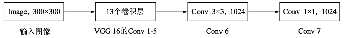
输入图像经过预处理后大小固定为300×300，首先经过backbone，本案例中使用的是VGG16网络的前13个卷积层，然后分别将VGG16的全连接层fc6和fc7转换成3 ×× 3卷积层block6和1 ×× 1卷积层block7，进一步提取特征。在block6中，使用了空洞数为6的空洞卷积，其padding也为6，这样做同样也是为了增加感受野的同时保持参数量与特征图尺寸的不变。

Extra Feature Layer

在VGG16的基础上，SSD进一步增加了4个深度卷积层，用于提取更高层的语义信息：

SSD-5

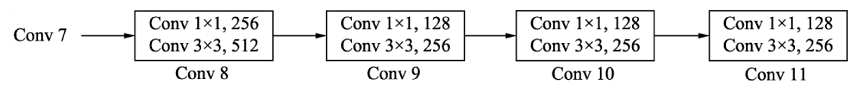
block8-11，用于更高语义信息的提取。block8的通道数为512，而block9、block10与block11的通道数都为256。从block7到block11，这5个卷积后输出特征图的尺寸依次为19×19、10×10、5×5、3×3和1×1。为了降低参数量，使用了1×1卷积先降低通道数为该层输出通道数的一半，再利用3×3卷积进行特征提取。

Anchor

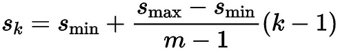
SSD采用了PriorBox来进行区域生成。将固定大小宽高的PriorBox作为先验的感兴趣区域，利用一个阶段完成能够分类与回归。设计大量的密集的PriorBox保证了对整幅图像的每个地方都有检测。PriorBox位置的表示形式是以中心点坐标和框的宽、高(cx,cy,w,h)来表示的，同时都转换成百分比的形式。 PriorBox生成规则： SSD由6个特征层来检测目标，在不同特征层上，PriorBox的尺寸scale大小是不一样的，最低层的scale=0.1，最高层的scale=0.95，其他层的计算公式如下：

SSD-6

在某个特征层上其scale一定，那么会设置不同长宽比ratio的PriorBox，其长和宽的计算公式如下：

在ratio=1的时候，还会根据该特征层和下一个特征层计算一个特定scale的PriorBox(长宽比ratio=1)，计算公式如下：

SSD-8

每个特征层的每个点都会以上述规则生成PriorBox，(cx,cy)由当前点的中心点来确定，由此每个特征层都生成大量密集的PriorBox，如下图：

SSD-9

SSD使用了第4、7、8、9、10和11这6个卷积层得到的特征图，这6个特征图尺寸越来越小，而其对应的感受野越来越大。6个特征图上的每一个点分别对应4、6、6、6、4、4个PriorBox。某个特征图上的一个点根据下采样率可以得到在原图的坐标，以该坐标为中心生成4个或6个不同大小的PriorBox，然后利用特征图的特征去预测每一个PriorBox对应类别与位置的预测量。例如：第8个卷积层得到的特征图大小为10×10×512，每个点对应6个PriorBox，一共有600个PriorBox。定义MultiBox类，生成多个预测框。

Detection Layer

SSD-10

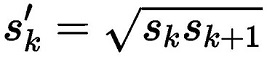
SSD模型一共有6个预测特征图，对于其中一个尺寸为m*n，通道为p的预测特征图，假设其每个像素点会产生k个anchor，每个anchor会对应c个类别和4个回归偏移量，使用(4+c)k个尺寸为3x3，通道为p的卷积核对该预测特征图进行卷积操作，得到尺寸为m*n，通道为(4+c)m*k的输出特征图，它包含了预测特征图上所产生的每个anchor的回归偏移量和各类别概率分数。所以对于尺寸为m*n的预测特征图，总共会产生(4+c)k*m*n个结果。cls分支的输出通道数为k*class_num，loc分支的输出通道数为k*4。

rom mindspore import nndef _make_layer(channels):in_channels = channels[0]layers = []for out_channels in channels[1:]:layers.append(nn.Conv2d(in_channels=in_channels, out_channels=out_channels, kernel_size=3))layers.append(nn.ReLU())in_channels = out_channelsreturn nn.SequentialCell(layers)class Vgg16(nn.Cell):"""VGG16 module."""def __init__(self):super(Vgg16, self).__init__()self.b1 = _make_layer([3, 64, 64])self.b2 = _make_layer([64, 128, 128])self.b3 = _make_layer([128, 256, 256, 256])self.b4 = _make_layer([256, 512, 512, 512])self.b5 = _make_layer([512, 512, 512, 512])self.m1 = nn.MaxPool2d(kernel_size=2, stride=2, pad_mode='SAME')self.m2 = nn.MaxPool2d(kernel_size=2, stride=2, pad_mode='SAME')self.m3 = nn.MaxPool2d(kernel_size=2, stride=2, pad_mode='SAME')self.m4 = nn.MaxPool2d(kernel_size=2, stride=2, pad_mode='SAME')self.m5 = nn.MaxPool2d(kernel_size=3, stride=1, pad_mode='SAME')def construct(self, x):# block1x = self.b1(x)x = self.m1(x)# block2x = self.b2(x)x = self.m2(x)# block3x = self.b3(x)x = self.m3(x)# block4x = self.b4(x)block4 = xx = self.m4(x)# block5x = self.b5(x)x = self.m5(x)return block4, x

import mindspore as ms
import mindspore.nn as nn
import mindspore.ops as opsdef _last_conv2d(in_channel, out_channel, kernel_size=3, stride=1, pad_mod='same', pad=0):in_channels = in_channelout_channels = in_channeldepthwise_conv = nn.Conv2d(in_channels, out_channels, kernel_size, stride, pad_mode='same',padding=pad, group=in_channels)conv = nn.Conv2d(in_channel, out_channel, kernel_size=1, stride=1, padding=0, pad_mode='same', has_bias=True)bn = nn.BatchNorm2d(in_channel, eps=1e-3, momentum=0.97,gamma_init=1, beta_init=0, moving_mean_init=0, moving_var_init=1)return nn.SequentialCell([depthwise_conv, bn, nn.ReLU6(), conv])class FlattenConcat(nn.Cell):"""FlattenConcat module."""def __init__(self):super(FlattenConcat, self).__init__()self.num_ssd_boxes = 8732def construct(self, inputs):output = ()batch_size = ops.shape(inputs[0])[0]for x in inputs:x = ops.transpose(x, (0, 2, 3, 1))output += (ops.reshape(x, (batch_size, -1)),)res = ops.concat(output, axis=1)return ops.reshape(res, (batch_size, self.num_ssd_boxes, -1))class MultiBox(nn.Cell):"""Multibox conv layers. Each multibox layer contains class conf scores and localization predictions."""def __init__(self):super(MultiBox, self).__init__()num_classes = 81out_channels = [512, 1024, 512, 256, 256, 256]num_default = [4, 6, 6, 6, 4, 4]loc_layers = []cls_layers = []for k, out_channel in enumerate(out_channels):loc_layers += [_last_conv2d(out_channel, 4 * num_default[k],kernel_size=3, stride=1, pad_mod='same', pad=0)]cls_layers += [_last_conv2d(out_channel, num_classes * num_default[k],kernel_size=3, stride=1, pad_mod='same', pad=0)]self.multi_loc_layers = nn.CellList(loc_layers)self.multi_cls_layers = nn.CellList(cls_layers)self.flatten_concat = FlattenConcat()def construct(self, inputs):loc_outputs = ()cls_outputs = ()for i in range(len(self.multi_loc_layers)):loc_outputs += (self.multi_loc_layers[i](inputs[i]),)cls_outputs += (self.multi_cls_layers[i](inputs[i]),)return self.flatten_concat(loc_outputs), self.flatten_concat(cls_outputs)class SSD300Vgg16(nn.Cell):"""SSD300Vgg16 module."""def __init__(self):super(SSD300Vgg16, self).__init__()# VGG16 backbone: block1~5self.backbone = Vgg16()# SSD blocks: block6~7self.b6_1 = nn.Conv2d(in_channels=512, out_channels=1024, kernel_size=3, padding=6, dilation=6, pad_mode='pad')self.b6_2 = nn.Dropout(p=0.5)self.b7_1 = nn.Conv2d(in_channels=1024, out_channels=1024, kernel_size=1)self.b7_2 = nn.Dropout(p=0.5)# Extra Feature Layers: block8~11self.b8_1 = nn.Conv2d(in_channels=1024, out_channels=256, kernel_size=1, padding=1, pad_mode='pad')self.b8_2 = nn.Conv2d(in_channels=256, out_channels=512, kernel_size=3, stride=2, pad_mode='valid')self.b9_1 = nn.Conv2d(in_channels=512, out_channels=128, kernel_size=1, padding=1, pad_mode='pad')self.b9_2 = nn.Conv2d(in_channels=128, out_channels=256, kernel_size=3, stride=2, pad_mode='valid')self.b10_1 = nn.Conv2d(in_channels=256, out_channels=128, kernel_size=1)self.b10_2 = nn.Conv2d(in_channels=128, out_channels=256, kernel_size=3, pad_mode='valid')self.b11_1 = nn.Conv2d(in_channels=256, out_channels=128, kernel_size=1)self.b11_2 = nn.Conv2d(in_channels=128, out_channels=256, kernel_size=3, pad_mode='valid')# boxesself.multi_box = MultiBox()def construct(self, x):# VGG16 backbone: block1~5block4, x = self.backbone(x)# SSD blocks: block6~7x = self.b6_1(x)  # 1024x = self.b6_2(x)x = self.b7_1(x)  # 1024x = self.b7_2(x)block7 = x# Extra Feature Layers: block8~11x = self.b8_1(x)  # 256x = self.b8_2(x)  # 512block8 = xx = self.b9_1(x)  # 128x = self.b9_2(x)  # 256block9 = xx = self.b10_1(x)  # 128x = self.b10_2(x)  # 256block10 = xx = self.b11_1(x)  # 128x = self.b11_2(x)  # 256block11 = x# boxesmulti_feature = (block4, block7, block8, block9, block10, block11)pred_loc, pred_label = self.multi_box(multi_feature)if not self.training:pred_label = ops.sigmoid(pred_label)pred_loc = pred_loc.astype(ms.float32)pred_label = pred_label.astype(ms.float32)return pred_loc, pred_label

损失函数

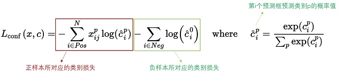
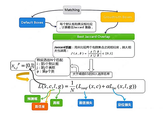
SSD算法的目标函数分为两部分：计算相应的预选框与目标类别的置信度误差（confidence loss, conf）以及相应的位置误差（locatization loss， loc）：

其中：
N 是先验框的正样本数量；
c 为类别置信度预测值;
l 为先验框的所对应边界框的位置预测值;
g 为ground truth的位置参数
α 用以调整confidence loss和location loss之间的比例，默认为1。

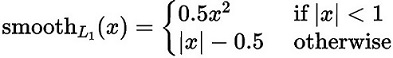
对于位置损失函数

针对所有的正样本，采用 Smooth L1 Loss, 位置信息都是 encode 之后的位置信息。

SSD-12

对于置信度损失函数

置信度损失是多类置信度(c)上的softmax损失。

SSD-13

def class_loss(logits, label):"""Calculate category losses."""label = ops.one_hot(label, ops.shape(logits)[-1], Tensor(1.0, ms.float32), Tensor(0.0, ms.float32))weight = ops.ones_like(logits)pos_weight = ops.ones_like(logits)sigmiod_cross_entropy = ops.binary_cross_entropy_with_logits(logits, label, weight.astype(ms.float32), pos_weight.astype(ms.float32))sigmoid = ops.sigmoid(logits)label = label.astype(ms.float32)p_t = label * sigmoid + (1 - label) * (1 - sigmoid)modulating_factor = ops.pow(1 - p_t, 2.0)alpha_weight_factor = label * 0.75 + (1 - label) * (1 - 0.75)focal_loss = modulating_factor * alpha_weight_factor * sigmiod_cross_entropyreturn focal_loss

Metrics

在SSD中，训练过程是不需要用到非极大值抑制(NMS)，但当进行检测时，例如输入一张图片要求输出框的时候，需要用到NMS过滤掉那些重叠度较大的预测框。
非极大值抑制的流程如下：

根据置信度得分进行排序
选择置信度最高的比边界框添加到最终输出列表中，将其从边界框列表中删除
计算所有边界框的面积
计算置信度最高的边界框与其它候选框的IoU
删除IoU大于阈值的边界框
重复上述过程，直至边界框列表为空

import json
from pycocotools.coco import COCO
from pycocotools.cocoeval import COCOevaldef apply_eval(eval_param_dict):net = eval_param_dict["net"]net.set_train(False)ds = eval_param_dict["dataset"]anno_json = eval_param_dict["anno_json"]coco_metrics = COCOMetrics(anno_json=anno_json,classes=train_cls,num_classes=81,max_boxes=100,nms_threshold=0.6,min_score=0.1)for data in ds.create_dict_iterator(output_numpy=True, num_epochs=1):img_id = data['img_id']img_np = data['image']image_shape = data['image_shape']# img_np shape: [batch_size, channels, height, width]# Convert it to [height, width, channels]#reshaped_image_data = np.transpose(img_np[0], (1, 2, 0))#reshaped_image_data = img_np.reshape(427, 640, 3)# Display the image using matplotlib#plt.imshow(reshaped_image_data)#plt.title(f"Image ID: {reshaped_image_data[0]}")#plt.show()output = net(Tensor(img_np))for batch_idx in range(img_np.shape[0]):pred_batch = {"boxes": output[0].asnumpy()[batch_idx],"box_scores": output[1].asnumpy()[batch_idx],"img_id": int(np.squeeze(img_id[batch_idx])),"image_shape": image_shape[batch_idx]}coco_metrics.update(pred_batch)eval_metrics = coco_metrics.get_metrics()return eval_metricsdef apply_nms(all_boxes, all_scores, thres, max_boxes):"""Apply NMS to bboxes."""y1 = all_boxes[:, 0]x1 = all_boxes[:, 1]y2 = all_boxes[:, 2]x2 = all_boxes[:, 3]areas = (x2 - x1 + 1) * (y2 - y1 + 1)order = all_scores.argsort()[::-1]keep = []while order.size > 0:i = order[0]keep.append(i)if len(keep) >= max_boxes:breakxx1 = np.maximum(x1[i], x1[order[1:]])yy1 = np.maximum(y1[i], y1[order[1:]])xx2 = np.minimum(x2[i], x2[order[1:]])yy2 = np.minimum(y2[i], y2[order[1:]])w = np.maximum(0.0, xx2 - xx1 + 1)h = np.maximum(0.0, yy2 - yy1 + 1)inter = w * hovr = inter / (areas[i] + areas[order[1:]] - inter)inds = np.where(ovr <= thres)[0]order = order[inds + 1]return keepclass COCOMetrics:"""Calculate mAP of predicted bboxes."""def __init__(self, anno_json, classes, num_classes, min_score, nms_threshold, max_boxes):self.num_classes = num_classesself.classes = classesself.min_score = min_scoreself.nms_threshold = nms_thresholdself.max_boxes = max_boxesself.val_cls_dict = {i: cls for i, cls in enumerate(classes)}self.coco_gt = COCO(anno_json)cat_ids = self.coco_gt.loadCats(self.coco_gt.getCatIds())self.class_dict = {cat['name']: cat['id'] for cat in cat_ids}self.predictions = []self.img_ids = []def update(self, batch):pred_boxes = batch['boxes']box_scores = batch['box_scores']img_id = batch['img_id']h, w = batch['image_shape']final_boxes = []final_label = []final_score = []self.img_ids.append(img_id)for c in range(1, self.num_classes):class_box_scores = box_scores[:, c]score_mask = class_box_scores > self.min_scoreclass_box_scores = class_box_scores[score_mask]class_boxes = pred_boxes[score_mask] * [h, w, h, w]if score_mask.any():nms_index = apply_nms(class_boxes, class_box_scores, self.nms_threshold, self.max_boxes)class_boxes = class_boxes[nms_index]class_box_scores = class_box_scores[nms_index]final_boxes += class_boxes.tolist()final_score += class_box_scores.tolist()final_label += [self.class_dict[self.val_cls_dict[c]]] * len(class_box_scores)for loc, label, score in zip(final_boxes, final_label, final_score):res = {}res['image_id'] = img_idres['bbox'] = [loc[1], loc[0], loc[3] - loc[1], loc[2] - loc[0]]res['score'] = scoreres['category_id'] = labelself.predictions.append(res)def get_metrics(self):with open('predictions.json', 'w') as f:json.dump(self.predictions, f)coco_dt = self.coco_gt.loadRes('predictions.json')E = COCOeval(self.coco_gt, coco_dt, iouType='bbox')E.params.imgIds = self.img_idsE.evaluate()E.accumulate()E.summarize()return E.stats[0]class SsdInferWithDecoder(nn.Cell):"""
SSD Infer wrapper to decode the bbox locations."""def __init__(self, network, default_boxes, ckpt_path):super(SsdInferWithDecoder, self).__init__()param_dict = ms.load_checkpoint(ckpt_path)ms.load_param_into_net(network, param_dict)self.network = networkself.default_boxes = default_boxesself.prior_scaling_xy = 0.1self.prior_scaling_wh = 0.2def construct(self, x):pred_loc, pred_label = self.network(x)default_bbox_xy = self.default_boxes[..., :2]default_bbox_wh = self.default_boxes[..., 2:]pred_xy = pred_loc[..., :2] * self.prior_scaling_xy * default_bbox_wh + default_bbox_xypred_wh = ops.exp(pred_loc[..., 2:] * self.prior_scaling_wh) * default_bbox_whpred_xy_0 = pred_xy - pred_wh / 2.0pred_xy_1 = pred_xy + pred_wh / 2.0pred_xy = ops.concat((pred_xy_0, pred_xy_1), -1)pred_xy = ops.maximum(pred_xy, 0)pred_xy = ops.minimum(pred_xy, 1)return pred_xy, pred_label

训练过程

（1）先验框匹配

在训练过程中，首先要确定训练图片中的ground truth（真实目标）与哪个先验框来进行匹配，与之匹配的先验框所对应的边界框将负责预测它。

SSD的先验框与ground truth的匹配原则主要有两点：

对于图片中每个ground truth，找到与其IOU最大的先验框，该先验框与其匹配，这样可以保证每个ground truth一定与某个先验框匹配。通常称与ground truth匹配的先验框为正样本，反之，若一个先验框没有与任何ground truth进行匹配，那么该先验框只能与背景匹配，就是负样本。
对于剩余的未匹配先验框，若某个ground truth的IOU大于某个阈值（一般是0.5），那么该先验框也与这个ground truth进行匹配。尽管一个ground truth可以与多个先验框匹配，但是ground truth相对先验框还是太少了，所以负样本相对正样本会很多。为了保证正负样本尽量平衡，SSD采用了hard negative mining，就是对负样本进行抽样，抽样时按照置信度误差（预测背景的置信度越小，误差越大）进行降序排列，选取误差的较大的top-k作为训练的负样本，以保证正负样本比例接近1:3。

注意点：

通常称与gt匹配的prior为正样本，反之，若某一个prior没有与任何一个gt匹配，则为负样本。
某个gt可以和多个prior匹配，而每个prior只能和一个gt进行匹配。
如果多个gt和某一个prior的IOU均大于阈值，那么prior只与IOU最大的那个进行匹配。

SSD-14

如上图所示，训练过程中的 prior boxes 和 ground truth boxes 的匹配，基本思路是：让每一个 prior box 回归并且到 ground truth box，这个过程的调控我们需要损失层的帮助，他会计算真实值和预测值之间的误差，从而指导学习的走向。

（2）损失函数

损失函数使用的是上文提到的位置损失函数和置信度损失函数的加权和。

（3）数据增强

使用之前定义好的数据增强方式，对创建好的数据增强方式进行数据增强。

模型训练时，设置模型训练的epoch次数为60，然后通过create_ssd_dataset类创建了训练集和验证集。batch_size大小为5，图像尺寸统一调整为300×300。损失函数使用位置损失函数和置信度损失函数的加权和，优化器使用Momentum，并设置初始学习率为0.001。回调函数方面使用了LossMonitor和TimeMonitor来监控训练过程中每个epoch结束后，损失值Loss的变化情况以及每个epoch、每个step的运行时间。设置每训练10个epoch保存一次模型。

import math
import itertools as itfrom mindspore import set_seedclass GeneratDefaultBoxes():"""Generate Default boxes for SSD, follows the order of (W, H, archor_sizes).`self.default_boxes` has a shape of [archor_sizes, H, W, 4], the last dimension is [y, x, h, w].`self.default_boxes_tlbr` has a shape as `self.default_boxes`, the last dimension is [y1, x1, y2, x2]."""def __init__(self):fk = 300 / np.array([8, 16, 32, 64, 100, 300])scale_rate = (0.95 - 0.1) / (len([4, 6, 6, 6, 4, 4]) - 1)scales = [0.1 + scale_rate * i for i in range(len([4, 6, 6, 6, 4, 4]))] + [1.0]self.default_boxes = []for idex, feature_size in enumerate([38, 19, 10, 5, 3, 1]):sk1 = scales[idex]sk2 = scales[idex + 1]sk3 = math.sqrt(sk1 * sk2)if idex == 0 and not [[2], [2, 3], [2, 3], [2, 3], [2], [2]][idex]:w, h = sk1 * math.sqrt(2), sk1 / math.sqrt(2)all_sizes = [(0.1, 0.1), (w, h), (h, w)]else:all_sizes = [(sk1, sk1)]for aspect_ratio in [[2], [2, 3], [2, 3], [2, 3], [2], [2]][idex]:w, h = sk1 * math.sqrt(aspect_ratio), sk1 / math.sqrt(aspect_ratio)all_sizes.append((w, h))all_sizes.append((h, w))all_sizes.append((sk3, sk3))assert len(all_sizes) == [4, 6, 6, 6, 4, 4][idex]for i, j in it.product(range(feature_size), repeat=2):for w, h in all_sizes:cx, cy = (j + 0.5) / fk[idex], (i + 0.5) / fk[idex]self.default_boxes.append([cy, cx, h, w])def to_tlbr(cy, cx, h, w):return cy - h / 2, cx - w / 2, cy + h / 2, cx + w / 2# For IoU calculationself.default_boxes_tlbr = np.array(tuple(to_tlbr(*i) for i in self.default_boxes), dtype='float32')self.default_boxes = np.array(self.default_boxes, dtype='float32')default_boxes_tlbr = GeneratDefaultBoxes().default_boxes_tlbr
default_boxes = GeneratDefaultBoxes().default_boxesy1, x1, y2, x2 = np.split(default_boxes_tlbr[:, :4], 4, axis=-1)
vol_anchors = (x2 - x1) * (y2 - y1)
matching_threshold = 0.5

from mindspore.common.initializer import initializer, TruncatedNormaldef init_net_param(network, initialize_mode='TruncatedNormal'):"""Init the parameters in net."""params = network.trainable_params()for p in params:if 'beta' not in p.name and 'gamma' not in p.name and 'bias' not in p.name:if initialize_mode == 'TruncatedNormal':p.set_data(initializer(TruncatedNormal(0.02), p.data.shape, p.data.dtype))else:p.set_data(initialize_mode, p.data.shape, p.data.dtype)def get_lr(global_step, lr_init, lr_end, lr_max, warmup_epochs, total_epochs, steps_per_epoch):""" generate learning rate array"""lr_each_step = []total_steps = steps_per_epoch * total_epochswarmup_steps = steps_per_epoch * warmup_epochsfor i in range(total_steps):if i < warmup_steps:lr = lr_init + (lr_max - lr_init) * i / warmup_stepselse:lr = lr_end + (lr_max - lr_end) * (1. + math.cos(math.pi * (i - warmup_steps) / (total_steps - warmup_steps))) / 2.if lr < 0.0:lr = 0.0lr_each_step.append(lr)current_step = global_steplr_each_step = np.array(lr_each_step).astype(np.float32)learning_rate = lr_each_step[current_step:]return learning_rate

import mindspore.dataset as ds
ds.config.set_enable_shared_mem(False)

import timefrom mindspore.amp import DynamicLossScalerset_seed(1)# load data
mindrecord_dir = "./datasets/MindRecord_COCO"
mindrecord_file = "./datasets/MindRecord_COCO/ssd.mindrecord0"dataset = create_ssd_dataset(mindrecord_file, batch_size=5, rank=0, use_multiprocessing=True)
dataset_size = dataset.get_dataset_size()image, get_loc, gt_label, num_matched_boxes = next(dataset.create_tuple_iterator())# Network definition and initialization
network = SSD300Vgg16()
init_net_param(network)# Define the learning rate
lr = Tensor(get_lr(global_step=0 * dataset_size,lr_init=0.001, lr_end=0.001 * 0.05, lr_max=0.05,warmup_epochs=2, total_epochs=60, steps_per_epoch=dataset_size))# Define the optimizer
opt = nn.Momentum(filter(lambda x: x.requires_grad, network.get_parameters()), lr,0.9, 0.00015, float(1024))# Define the forward procedure
def forward_fn(x, gt_loc, gt_label, num_matched_boxes):pred_loc, pred_label = network(x)mask = ops.less(0, gt_label).astype(ms.float32)num_matched_boxes = ops.sum(num_matched_boxes.astype(ms.float32))# Positioning lossmask_loc = ops.tile(ops.expand_dims(mask, -1), (1, 1, 4))smooth_l1 = nn.SmoothL1Loss()(pred_loc, gt_loc) * mask_locloss_loc = ops.sum(ops.sum(smooth_l1, -1), -1)# Category lossloss_cls = class_loss(pred_label, gt_label)loss_cls = ops.sum(loss_cls, (1, 2))return ops.sum((loss_cls + loss_loc) / num_matched_boxes)grad_fn = ms.value_and_grad(forward_fn, None, opt.parameters, has_aux=False)
loss_scaler = DynamicLossScaler(1024, 2, 1000)# Gradient updates
def train_step(x, gt_loc, gt_label, num_matched_boxes):loss, grads = grad_fn(x, gt_loc, gt_label, num_matched_boxes)opt(grads)return lossprint("=================== Starting Training =====================")
for epoch in range(60):network.set_train(True)begin_time = time.time()for step, (image, get_loc, gt_label, num_matched_boxes) in enumerate(dataset.create_tuple_iterator()):loss = train_step(image, get_loc, gt_label, num_matched_boxes)end_time = time.time()times = end_time - begin_timeprint(f"Epoch:[{int(epoch + 1)}/{int(60)}], "f"loss:{loss} , "f"time:{times}s ")
ms.save_checkpoint(network, "ssd-60_9.ckpt")
print("=================== Training Success =====================")

=================== Starting Training =====================
Epoch:[1/60], loss:1084.1497 , time:268.41673254966736s 
Epoch:[2/60], loss:1074.2557 , time:1.8542943000793457s 
Epoch:[3/60], loss:1056.8948 , time:1.8581438064575195s 
Epoch:[4/60], loss:1038.4043 , time:2.5073862075805664s 
Epoch:[5/60], loss:1019.4508 , time:1.6549866199493408s 
Epoch:[6/60], loss:1000.02734 , time:1.8116443157196045s 
Epoch:[7/60], loss:979.87933 , time:1.7282652854919434s 
Epoch:[8/60], loss:958.61566 , time:1.7475194931030273s 
Epoch:[9/60], loss:935.74896 , time:1.6405341625213623s 
Epoch:[10/60], loss:910.70667 , time:1.7443654537200928s 
Epoch:[11/60], loss:882.87103 , time:1.6887924671173096s 
Epoch:[12/60], loss:851.63904 , time:1.8271369934082031s 
Epoch:[13/60], loss:816.519 , time:1.722499132156372s 
Epoch:[14/60], loss:777.2507 , time:1.7766461372375488s 
Epoch:[15/60], loss:733.9753 , time:1.7010409832000732s 
Epoch:[16/60], loss:687.3042 , time:1.7122321128845215s 
Epoch:[17/60], loss:638.4035 , time:1.769655704498291s 
Epoch:[18/60], loss:588.79944 , time:1.652649164199829s 
Epoch:[19/60], loss:540.2302 , time:2.1968443393707275s 
Epoch:[20/60], loss:494.28754 , time:1.7006897926330566s 
Epoch:[21/60], loss:452.18365 , time:1.6936073303222656s 
Epoch:[22/60], loss:414.63162 , time:1.7576310634613037s 
Epoch:[23/60], loss:381.84366 , time:1.7209653854370117s 
Epoch:[24/60], loss:353.64685 , time:1.7930691242218018s 
Epoch:[25/60], loss:329.64752 , time:2.043553113937378s 
Epoch:[26/60], loss:309.32376 , time:1.9476304054260254s 
Epoch:[27/60], loss:292.14877 , time:1.797055959701538s 
Epoch:[28/60], loss:277.5957 , time:1.7137107849121094s 
Epoch:[29/60], loss:265.23407 , time:1.723273754119873s 
Epoch:[30/60], loss:254.72319 , time:1.8662052154541016s 
Epoch:[31/60], loss:245.69922 , time:1.705491065979004s 
Epoch:[32/60], loss:237.95853 , time:1.6677360534667969s 
Epoch:[33/60], loss:231.26953 , time:1.7562761306762695s 
Epoch:[34/60], loss:225.46909 , time:1.707484483718872s 
Epoch:[35/60], loss:220.4212 , time:1.74747896194458s 
Epoch:[36/60], loss:216.0148 , time:1.7244234085083008s 
Epoch:[37/60], loss:212.17128 , time:1.694749355316162s 
Epoch:[38/60], loss:208.79092 , time:1.7968826293945312s 
Epoch:[39/60], loss:205.83005 , time:1.7690155506134033s 
Epoch:[40/60], loss:203.2412 , time:1.7921578884124756s 
Epoch:[41/60], loss:200.95876 , time:1.7308340072631836s 
Epoch:[42/60], loss:198.97131 , time:1.838721513748169s 
Epoch:[43/60], loss:197.22264 , time:1.8696863651275635s 
Epoch:[44/60], loss:195.71373 , time:1.8561134338378906s 
Epoch:[45/60], loss:194.39456 , time:1.7734193801879883s 
Epoch:[46/60], loss:193.25168 , time:1.838977575302124s 
Epoch:[47/60], loss:192.2803 , time:1.7496910095214844s 
Epoch:[48/60], loss:191.45642 , time:1.8346962928771973s 
Epoch:[49/60], loss:190.76175 , time:1.716414451599121s 
Epoch:[50/60], loss:190.17783 , time:1.6865875720977783s 
Epoch:[51/60], loss:189.7042 , time:1.7670023441314697s 
Epoch:[52/60], loss:189.32454 , time:1.8355705738067627s 
Epoch:[53/60], loss:189.02377 , time:1.785146713256836s 
Epoch:[54/60], loss:188.79697 , time:2.1677238941192627s 
Epoch:[55/60], loss:188.63405 , time:1.7368669509887695s 
Epoch:[56/60], loss:188.51495 , time:1.6919987201690674s 
Epoch:[57/60], loss:188.44801 , time:1.7100017070770264s 
Epoch:[58/60], loss:188.4046 , time:1.692232608795166s 
Epoch:[59/60], loss:188.38766 , time:1.7659671306610107s 
Epoch:[60/60], loss:188.37616 , time:1.6955435276031494s 
=================== Training Success =====================

评估

自定义eval_net()类对训练好的模型进行评估，调用了上述定义的SsdInferWithDecoder类返回预测的坐标及标签，然后分别计算了在不同的IoU阈值、area和maxDets设置下的Average Precision（AP）和Average Recall（AR）。使用COCOMetrics类计算mAP。模型在测试集上的评估指标如下。

精确率（AP）和召回率（AR）的解释

TP：IoU>设定的阈值的检测框数量（同一Ground Truth只计算一次）。
FP：IoU<=设定的阈值的检测框，或者是检测到同一个GT的多余检测框的数量。
FN：没有检测到的GT的数量。

精确率（AP）和召回率（AR）的公式

精确率（Average Precision,AP）：

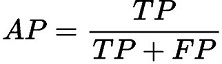
精确率是将正样本预测正确的结果与正样本预测的结果和预测错误的结果的和的比值，主要反映出预测结果错误率。
召回率（Average Recall,AR）：

召回率是正样本预测正确的结果与正样本预测正确的结果和正样本预测错误的和的比值，主要反映出来的是预测结果中的漏检率。

关于以下代码运行结果的输出指标

第一个值即为mAP(mean Average Precision), 即各类别AP的平均值。
第二个值是iou取0.5的mAP值，是voc的评判标准。
第三个值是评判较为严格的mAP值，可以反应算法框的位置精准程度；中间几个数为物体大小的mAP值。

对于AR看一下maxDets=10/100的mAR值，反应检出率，如果两者接近，说明对于这个数据集来说，不用检测出100个框，可以提高性能。

mindrecord_file = "./datasets/MindRecord_COCO/ssd_eval.mindrecord0"def ssd_eval(dataset_path, ckpt_path, anno_json):"""SSD evaluation."""batch_size = 1ds = create_ssd_dataset(dataset_path, batch_size=batch_size,is_training=False, use_multiprocessing=False)network = SSD300Vgg16()print("Load Checkpoint!")net = SsdInferWithDecoder(network, Tensor(default_boxes), ckpt_path)net.set_train(False)total = ds.get_dataset_size() * batch_sizeprint("\n========================================\n")print("total images num: ", total)eval_param_dict = {"net": net, "dataset": ds, "anno_json": anno_json}mAP = apply_eval(eval_param_dict)print("\n========================================\n")print(f"mAP: {mAP}")def eval_net():print("Start Eval!")ssd_eval(mindrecord_file, "./ssd-60_9.ckpt", anno_json)eval_net()

Start Eval!
Load Checkpoint!========================================total images num:  9
loading annotations into memory...
Done (t=0.00s)
creating index...
index created!
Loading and preparing results...
DONE (t=1.17s)
creating index...
index created!
Running per image evaluation...
Evaluate annotation type *bbox*
DONE (t=1.28s).
Accumulating evaluation results...
DONE (t=0.37s).Average Precision  (AP) @[ IoU=0.50:0.95 | area=   all | maxDets=100 ] = 0.008Average Precision  (AP) @[ IoU=0.50      | area=   all | maxDets=100 ] = 0.016Average Precision  (AP) @[ IoU=0.75      | area=   all | maxDets=100 ] = 0.001Average Precision  (AP) @[ IoU=0.50:0.95 | area= small | maxDets=100 ] = 0.000Average Precision  (AP) @[ IoU=0.50:0.95 | area=medium | maxDets=100 ] = 0.006Average Precision  (AP) @[ IoU=0.50:0.95 | area= large | maxDets=100 ] = 0.028Average Recall     (AR) @[ IoU=0.50:0.95 | area=   all | maxDets=  1 ] = 0.021Average Recall     (AR) @[ IoU=0.50:0.95 | area=   all | maxDets= 10 ] = 0.042Average Recall     (AR) @[ IoU=0.50:0.95 | area=   all | maxDets=100 ] = 0.071Average Recall     (AR) @[ IoU=0.50:0.95 | area= small | maxDets=100 ] = 0.000Average Recall     (AR) @[ IoU=0.50:0.95 | area=medium | maxDets=100 ] = 0.063Average Recall     (AR) @[ IoU=0.50:0.95 | area= large | maxDets=100 ] = 0.303========================================mAP: 0.007964928263322426

引用¶

[1] Liu W, Anguelov D, Erhan D, et al. Ssd: Single shot multibox detector[C]//European conference on computer vision. Springer, Cham, 2016: 21-37.

经过数据预处理、模型构建、定义损失函数后，训练模型。（没有看太懂）

与动手学深度学习中的单发多框检测（SSD）相比似乎Anchor处理得更精细。

模型的评估结果mAP: 0.007964928263322426似乎太小了。（课程的开始说使用Nvidia Titan X在VOC 2007测试集上，SSD对于输入尺寸300x300的网络，达到74.3%mAP(mean Average Precision)以及59FPS；对于512x512的网络，达到了76.9%mAP ，超越当时最强的Faster RCNN(73.2%mAP)。）