【Machine Learning】8.逻辑回归及其在分类问题的应用
逻辑回归及其在分类问题的应用
- 1. 导入
- 2.Sigmoid函数
- 3.逻辑回归
- 4.分类问题示例及决策边界
- 4.1 导入
- 4.2 数据集
- 4.3 模型应用
- Refresher on logistic regression and decision boundary
- Plotting decision boundary
在分类问题之前,我们要知道sigmoid函数,以及逻辑回归是sigmoid函数在线性回归上的应用
1. 导入
import numpy as np
%matplotlib widget
import matplotlib.pyplot as plt
from plt_one_addpt_onclick import plt_one_addpt_onclick
from lab_utils_common import draw_vthresh
plt.style.use('./deeplearning.mplstyle')
2.Sigmoid函数
在分类时,我们希望分类模型的预测值介于0和1之间,因为我们的输出变量
y
y
y是0或1,而sigmoid函数可以把输出值压缩到0-1
g
(
z
)
=
1
1
+
e
−
z
(1)
g(z) = \frac{1}{1+e^{-z}}\tag{1}
g(z)=1+e−z1(1)
在逻辑回归的情况下,z(sigmoid函数的输入)是线性回归模型的输出。
- 在单个示例中, z z z是标量。
- 在多个示例的情况下, z z z可以是由 m m m值组成的向量,每个示例对应一个值。
- sigmoid函数的实现应涵盖这两种潜在的输入格式。
numpy自带exp函数可以把array中的数取 e z e^z ez,其中z为array中的数
# Input is an array.
input_array = np.array([1,2,3])
exp_array = np.exp(input_array)

print("Input to exp:", input_array)
print("Output of exp:", exp_array)

# Input is a single number
input_val = 1
exp_val = np.exp(input_val)

print("Input to exp:", input_val)
print("Output of exp:", exp_val)


Input to exp: [1 2 3]
Output of exp: [ 2.718  7.389 20.086]
Input to exp: 1
Output of exp: 2.718281828459045
手撕sigmoid(很简单)
def sigmoid(z):
    """
    Compute the sigmoid of z

    Args:
        z (ndarray): A scalar, numpy array of any size.

    Returns:
        g (ndarray): sigmoid(z), with the same shape as z

    """

    g = 1/(1+np.exp(-z))

    return g
对比一下处理前后的数据
# Generate an array of evenly spaced values between -10 and 10
z_tmp = np.arange(-10,11)

# Use the function implemented above to get the sigmoid values
y = sigmoid(z_tmp)

# Code for pretty printing the two arrays next to each other
np.set_printoptions(precision=3)
print("Input (z), Output (sigmoid(z))")
print(np.c_[z_tmp, y])


Input (z), Output (sigmoid(z))
[[-1.000e+01  4.540e-05]
 [-9.000e+00  1.234e-04]
 [-8.000e+00  3.354e-04]
 [-7.000e+00  9.111e-04]
 [-6.000e+00  2.473e-03]
 [-5.000e+00  6.693e-03]
 [-4.000e+00  1.799e-02]
 [-3.000e+00  4.743e-02]
 [-2.000e+00  1.192e-01]
 [-1.000e+00  2.689e-01]
 [ 0.000e+00  5.000e-01]
 [ 1.000e+00  7.311e-01]
 [ 2.000e+00  8.808e-01]
 [ 3.000e+00  9.526e-01]
 [ 4.000e+00  9.820e-01]
 [ 5.000e+00  9.933e-01]
 [ 6.000e+00  9.975e-01]
 [ 7.000e+00  9.991e-01]
 [ 8.000e+00  9.997e-01]
 [ 9.000e+00  9.999e-01]
 [ 1.000e+01  1.000e+00]]
至于np.c_,可以看看numpy.c_
array将在升级到至少二维后沿其最后一个轴堆叠
np.c_[np.array([1,2,3]), np.array([4,5,6])]
array([[1, 4],
       [2, 5],
       [3, 6]])


np.c_[np.array([[1,2,3]]), 0, 0, np.array([[4,5,6]])]
array([[1, 2, 3, ..., 4, 5, 6]])
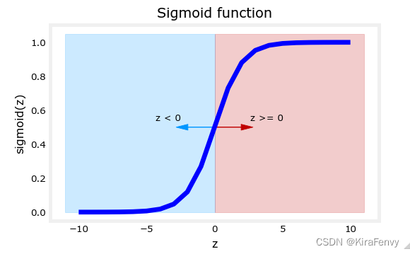
绘制z与sigmoid(z)的图像
# Plot z vs sigmoid(z)
fig,ax = plt.subplots(1,1,figsize=(5,3))
ax.plot(z_tmp, y, c="b")

ax.set_title("Sigmoid function")
ax.set_ylabel('sigmoid(z)')
ax.set_xlabel('z')
draw_vthresh(ax,0)
3.逻辑回归
如果w和x是向量:
f
w
,
b
(
x
(
i
)
)
=
g
(
w
⋅
x
(
i
)
+
b
)
(2)
f_{\mathbf{w},b}(\mathbf{x}^{(i)}) = g(\mathbf{w} \cdot \mathbf{x}^{(i)} + b ) \tag{2}
fw,b(x(i))=g(w⋅x(i)+b)(2)
sigmoid依然是:
g
(
z
)
=
1
1
+
e
−
z
(3)
g(z) = \frac{1}{1+e^{-z}}\tag{3}
g(z)=1+e−z1(3)
只是z的算法有变化:
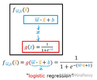
此时就是逻辑回归模型,是将sigmoid运用到线性回归上的模型
4.分类问题示例及决策边界
我们要通过逻辑回归来获取分类问题的决策边界
4.1 导入
import numpy as np
%matplotlib widget
import matplotlib.pyplot as plt
from lab_utils_common import plot_data, sigmoid, draw_vthresh
plt.style.use('./deeplearning.mplstyle')
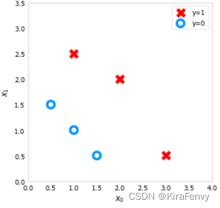
4.2 数据集
X = np.array([[0.5, 1.5], [1,1], [1.5, 0.5], [3, 0.5], [2, 2], [1, 2.5]])
y = np.array([0, 0, 0, 1, 1, 1]).reshape(-1,1)
fig,ax = plt.subplots(1,1,figsize=(4,4))
plot_data(X, y, ax)

ax.axis([0, 4, 0, 3.5])
ax.set_ylabel('$x_1$')
ax.set_xlabel('$x_0$')
plt.show()
4.3 模型应用
-
假设我们的决策边界直线形如
f ( x ) = g ( w 0 x 0 + w 1 x 1 + b ) f(x) = g(w_0x_0+w_1x_1 + b) f(x)=g(w0x0+w1x1+b)
where g ( z ) = 1 1 + e − z g(z) = \frac{1}{1+e^{-z}} g(z)=1+e−z1, which is the sigmoid function
-
假设我们拟合,得出的最优解 b = − 3 , w 0 = 1 , w 1 = 1 b = -3, w_0 = 1, w_1 = 1 b=−3,w0=1,w1=1.,拟合的方法我们后面会谈到
f ( x ) = g ( x 0 + x 1 − 3 ) f(x) = g(x_0+x_1-3) f(x)=g(x0+x1−3)
(You’ll learn how to fit these parameters to the data further in the course)
Refresher on logistic regression and decision boundary
-
Recall that for logistic regression, the model is represented as
f w , b ( x ( i ) ) = g ( w ⋅ x ( i ) + b ) (1) f_{\mathbf{w},b}(\mathbf{x}^{(i)}) = g(\mathbf{w} \cdot \mathbf{x}^{(i)} + b) \tag{1} fw,b(x(i))=g(w⋅x(i)+b)(1)
where g ( z ) g(z) g(z) is known as the sigmoid function and it maps all input values to values between 0 and 1:
g ( z ) = 1 1 + e − z (2) g(z) = \frac{1}{1+e^{-z}}\tag{2} g(z)=1+e−z1(2)
and w ⋅ x \mathbf{w} \cdot \mathbf{x} w⋅x is the vector dot product:w ⋅ x = w 0 x 0 + w 1 x 1 \mathbf{w} \cdot \mathbf{x} = w_0 x_0 + w_1 x_1 w⋅x=w0x0+w1x1
-
We interpret the output of the model ( f w , b ( x ) f_{\mathbf{w},b}(x) fw,b(x)) as the probability that y = 1 y=1 y=1 given x x x and parameterized by w w w and b b b.
-
Therefore, to get a final prediction ( y = 0 y=0 y=0 or y = 1 y=1 y=1) from the logistic regression model, we can use the following heuristic -
if f w , b ( x ) > = 0.5 f_{\mathbf{w},b}(x) >= 0.5 fw,b(x)>=0.5, predict y = 1 y=1 y=1
if f w , b ( x ) < 0.5 f_{\mathbf{w},b}(x) < 0.5 fw,b(x)<0.5, predict y = 0 y=0 y=0
-
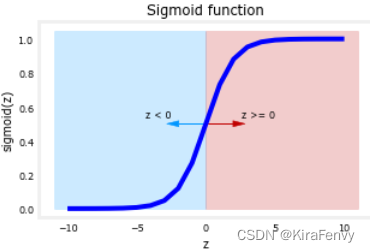
Let’s plot the sigmoid function to see where g ( z ) > = 0.5 g(z) >= 0.5 g(z)>=0.5
# Plot sigmoid(z) over a range of values from -10 to 10
z = np.arange(-10,11)

fig,ax = plt.subplots(1,1,figsize=(5,3))
# Plot z vs sigmoid(z)
ax.plot(z, sigmoid(z), c="b")

ax.set_title("Sigmoid function")
ax.set_ylabel('sigmoid(z)')
ax.set_xlabel('z')
draw_vthresh(ax,0)
-
As you can see, g ( z ) > = 0.5 g(z) >= 0.5 g(z)>=0.5 for z > = 0 z >=0 z>=0
-
For a logistic regression model, z = w ⋅ x + b z = \mathbf{w} \cdot \mathbf{x} + b z=w⋅x+b. Therefore,
if w ⋅ x + b > = 0 \mathbf{w} \cdot \mathbf{x} + b >= 0 w⋅x+b>=0, the model predicts y = 1 y=1 y=1
if w ⋅ x + b < 0 \mathbf{w} \cdot \mathbf{x} + b < 0 w⋅x+b<0, the model predicts y = 0 y=0 y=0
Plotting decision boundary
-
Our logistic regression model has the form
f ( x ) = g ( − 3 + x 0 + x 1 ) f(x) = g(-3 + x_0+x_1) f(x)=g(−3+x0+x1)
-
From what you’ve learnt above, you can see that this model predicts y = 1 y=1 y=1 if − 3 + x 0 + x 1 > = 0 -3 + x_0+x_1 >= 0 −3+x0+x1>=0
Let’s see what this looks like graphically. We’ll start by plotting − 3 + x 0 + x 1 = 0 -3 + x_0+x_1 = 0 −3+x0+x1=0, which is equivalent to x 1 = 3 − x 0 x_1 = 3 - x_0 x1=3−x0.
# Choose values between 0 and 6
x0 = np.arange(0,6)

x1 = 3 - x0
fig,ax = plt.subplots(1,1,figsize=(5,4))
# Plot the decision boundary
ax.plot(x0,x1, c="b")
ax.axis([0, 4, 0, 3.5])

# Fill the region below the line
ax.fill_between(x0,x1, alpha=0.2)

# Plot the original data
plot_data(X,y,ax)
ax.set_ylabel(r'$x_1$')
ax.set_xlabel(r'$x_0$')
plt.show()
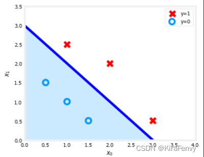
后面使用高次多项式,会看到非线性边界