Pytorch入门基础知识(一)
目录
一、Tensor的基本定义
二、Tensor的类型
三、Tensor常用函数
3.1 Tensor创建相关函数
3.2 Tensor的属性
3.3 Tensor加法运算
3.4 减法运算
3.5 乘法运算
3.6 除法运算
3.7 矩阵运算
3.8 指数运算
3.9 对数运算
3.10 开方运算
三、Pytorch中的广播机制
四、Pytorch中的基本操作
4.1 Pytorch取整、取余相关函数
4.2 pytorch中的三角函数&其他常用函数
4.3 Pytorch比较运算符
4.4 pytorch排序相关函数
一、Tensor的基本定义
张量(tensor)是pytorch中最基础的一种数据结构 ,在pytorch中的操作都是基于tensor。我们可能对标量,向量,矩阵都非常熟悉,其实张量是标量、矩阵等更为高维、更为普遍的表现形式。

二、Tensor的类型
在 torch 中 分为CUP 存储运算的tensor和 GPU存储运算的张量。Tensor在cpu、gpu下分别有 8 种数据类型,其中默认的数据类型为 32 位浮点型
| 数据类型 | dtype | CPU Tensor | GPU Tensor |
| 16 位浮点型 | torch.float16 或 torch.half | torch.HalfTensor | torch.cuda.HalfTensor |
| 32 位浮点型 | torch.float32 或 torch.float | torch.FloatTensor | torch.cuda.FloatTensor |
| 64 位浮点型 | torch.float64 或 torch.double | torch.DoubleTensor | torch.cuda.DoubleTensor |
| 8 位无符号整型 | torch.uint8 | torch.ByteTensor | torch.cuda.ByteTensor |
| 8 位有符号整型 | torch.int8 | torch.CharTensor | torch.cuda.CharTensor |
| 16 位有符号整型 | torch.int16 或 torch.short | torch.ShortTensor | torch.cuda.ShortTensor |
| 32 位有符号整型 | torch.int32 或 torch.int | torch.IntTensor | torch.cuda.IntTensor |
| 64 位有符号整型 | torch.int64 或 torch.long | torch.LongTensor | torch.cuda.LongTensor |
三、Tensor常用函数

3.1 Tensor创建相关函数
import torch
#直接使用数据初始化一个张量
a=torch.Tensor([[1,2,4],[4,9,3],[2,7,5]])
print(a)
print(a.type())
#直接规定张量形状的方式来定义一个tensor
b=torch.Tensor(4,5)
print(b)
print(b.type())

#定义元素全是1的张量
c=torch.ones(2,3)
print(c)
print(c.type())

#定义对角线全是1的张量
d=torch.eye(3,4)
print(d)
print(d.type())

#定于元素全是0的张量
e=torch.zeros(4,5)
print(e)

f=torch.Tensor([[1,7,3],
               [4,5,0]])
#定义类张量f、元素全为1的Tensor
print(torch.ones_like(f))
#定义类张量f、元素全为0的Tensor
print(torch.zeros_like(f))

#随机生成Tensor
g=torch.rand(4,6)
print(g)
tensor([[1., 2., 4.],
[4., 9., 3.],
[2., 7., 5.]])
torch.FloatTensor
tensor([[0.0000e+00, 1.8750e+00, 0.0000e+00, 2.0000e+00, 0.0000e+00],
[2.2500e+00, 0.0000e+00, 2.2500e+00, 0.0000e+00, 2.5312e+00],
[0.0000e+00, 2.1250e+00, 0.0000e+00, 2.0000e+00, 0.0000e+00],
[2.4375e+00, 0.0000e+00, 2.3125e+00, 8.4490e-39, 1.0194e-38]])
torch.FloatTensor
tensor([[1., 1., 1.],
[1., 1., 1.]])
torch.FloatTensor
tensor([[1., 0., 0., 0.],
[0., 1., 0., 0.],
[0., 0., 1., 0.]])
torch.FloatTensor
tensor([[0., 0., 0., 0., 0.],
[0., 0., 0., 0., 0.],
[0., 0., 0., 0., 0.],
[0., 0., 0., 0., 0.]])
tensor([[1., 1., 1.],
[1., 1., 1.]])
tensor([[0., 0., 0.],
[0., 0., 0.]])
tensor([[0.5883, 0.6820, 0.1486, 0.1378, 0.2527, 0.9632],
[0.1268, 0.8534, 0.8985, 0.4486, 0.4386, 0.0506],
[0.8461, 0.1896, 0.2956, 0.7772, 0.0755, 0.1335],
[0.8106, 0.9190, 0.2299, 0.3782, 0.6713, 0.8427]])
下面重点看一下
torch.normal()函数
官方文档给出的解释是返回一个张量,张量里面的随机数是从相互独立的正态分布中随机生成的。举一个例子来解释一下
为了防止列举的例子太过隐晦难懂,先复习一下 torch.arange()函数的用法
print(torch.arange(1.,11.))
'''
运行结果
tensor([ 1.,  2.,  3.,  4.,  5.,  6.,  7.,  8.,  9., 10.])
'''
print(torch.arange(1,0,-0.1))
'''
运行结果
tensor([1.0000, 0.9000, 0.8000, 0.7000,
0.6000, 0.5000, 0.4000, 0.3000, 0.2000,
0.1000])
'''
a=torch.normal(mean=torch.arange(1.,11.),std=torch.arange(1,0,-0.1))
print(a)
'''
运行结果
tensor([ 1.6596,  2.2340,  2.9046,  3.7704,
  4.8815,  4.8456,  7.2505,  7.9999,
         8.8839, 10.0721])

'''
1.6596,#是从均值为1,标准差为1的正态分布中随机生成的
2.2340, #是从均值为2,标准差为0.9的正态分布中随机生成的
2.9046, #是从均值为3,标准差为0.8的正态分布中随机生成的
3.7704, #后面依次类推
4.8815,
4.8456,
7.2505,
7.9999,
8.8839,
10.0721
3.2 Tensor的属性
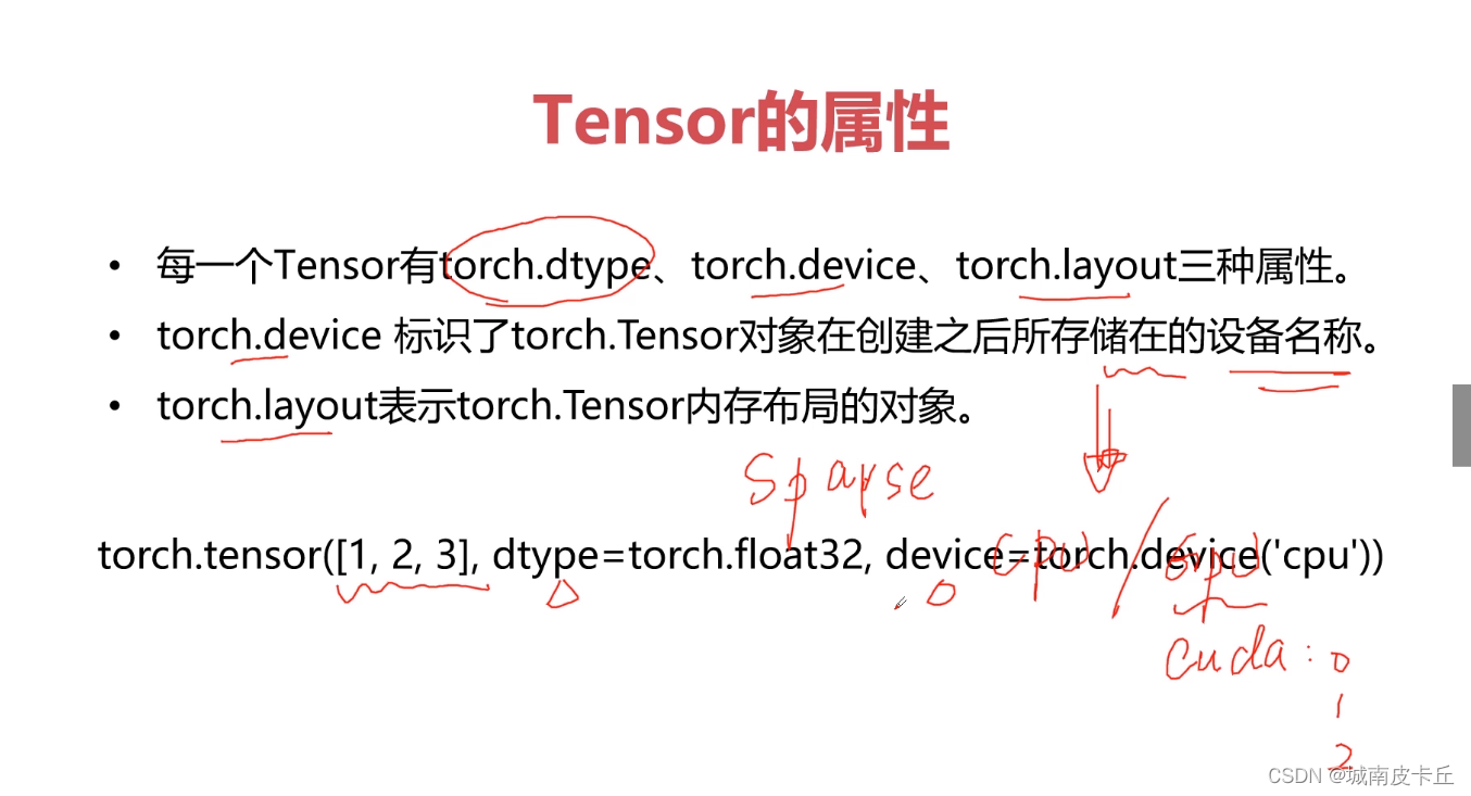
>>>a=torch.Tensor([2,2],device=torch.device('cpu'))
>>>a
tensor([2., 2.])
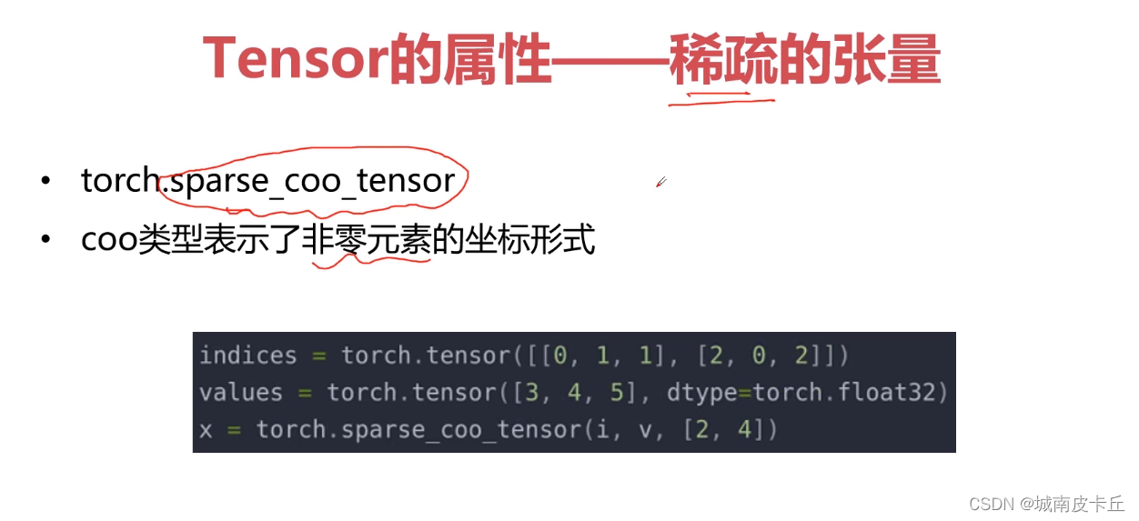
i=torch.Tensor([[0,1,2,3],[0,1,2,3]])
v=torch.Tensor([1,2,3,4])
a=torch.sparse_coo_tensor(i,v,(4,4)).to_dense()
print(a)
'''
result:
tensor([[1., 0., 0., 0.],
        [0., 2., 0., 0.],
        [0., 0., 3., 0.],
        [0., 0., 0., 4.]])
'''
3.3 Tensor加法运算
a=torch.rand(2,3)
b=torch.rand(2,3)
#tensor加法运算
print('a>>>{}'.format(a))
print('b>>>{}'.format(b))

print('a+b>>>{}'.format(a+b))
print('a.add(b)>>>{}'.format(a.add(b)))
print('torch.add(a,b)>>>{}'.format(torch.add(a,b)))
print('a>>>{}'.format(a))
print('a.add_(b)>>>{}'.format(a.add_(b)))#会改变a的值
print('a>>>{}'.format(a))
'''
result:

a>>>tensor([[0.8988, 0.5446, 0.5518],
        [0.9732, 0.9988, 0.4388]])
b>>>tensor([[0.5444, 0.1172, 0.0646],
        [0.7828, 0.4502, 0.6519]])
a+b>>>tensor([[1.4432, 0.6618, 0.6164],
        [1.7560, 1.4491, 1.0908]])
a.add(b)>>>tensor([[1.4432, 0.6618, 0.6164],
        [1.7560, 1.4491, 1.0908]])
torch.add(a,b)>>>tensor([[1.4432, 0.6618, 0.6164],
        [1.7560, 1.4491, 1.0908]])
a>>>tensor([[0.8988, 0.5446, 0.5518],
        [0.9732, 0.9988, 0.4388]])
a.add_(b)>>>tensor([[1.4432, 0.6618, 0.6164],
        [1.7560, 1.4491, 1.0908]])
a>>>tensor([[1.4432, 0.6618, 0.6164],
        [1.7560, 1.4491, 1.0908]])
'''
3.4 减法运算
a=torch.rand(2,3)
b=torch.rand(2,3)
#tensor减法运算
print('a>>>{}'.format(a))
print('b>>>{}'.format(b))

print('a-b>>>{}'.format(a-b))
print('a.sub(b)>>>{}'.format(a.sub(b)))
print('torch.sub(a,b)>>>{}'.format(torch.sub(a,b)))
print('a>>>{}'.format(a))
print('a.sub_(b)>>>{}'.format(a.sub_(b)))#会改变a的值
print('a>>>{}'.format(a))
'''
result:

a>>>tensor([[0.5074, 0.2774, 0.2372],
        [0.8903, 0.3377, 0.2094]])
b>>>tensor([[0.8004, 0.8801, 0.0041],
        [0.9146, 0.6384, 0.6574]])
a-b>>>tensor([[-0.2931, -0.6027,  0.2331],
        [-0.0244, -0.3007, -0.4479]])
a.sub(b)>>>tensor([[-0.2931, -0.6027,  0.2331],
        [-0.0244, -0.3007, -0.4479]])
torch.sub(a,b)>>>tensor([[-0.2931, -0.6027,  0.2331],
        [-0.0244, -0.3007, -0.4479]])
a>>>tensor([[0.5074, 0.2774, 0.2372],
        [0.8903, 0.3377, 0.2094]])
a.sub_(b)>>>tensor([[-0.2931, -0.6027,  0.2331],
        [-0.0244, -0.3007, -0.4479]])
a>>>tensor([[-0.2931, -0.6027,  0.2331],
        [-0.0244, -0.3007, -0.4479]])
'''
3.5 乘法运算
a=torch.rand(2,3)
b=torch.rand(2,3)
#tensor乘法运算
print('a>>>{}'.format(a))
print('b>>>{}'.format(b))

print('a*b>>>{}'.format(a*b))
print('a.mul(b)>>>{}'.format(a.mul(b)))
print('torch.mul(a,b)>>>{}'.format(torch.mul(a,b)))
print('a>>>{}'.format(a))
print('a.mul_(b)>>>{}'.format(a.mul_(b)))#会改变a的值
print('a>>>{}'.format(a))
'''
result:

a>>>tensor([[0.6919, 0.9733, 0.2953],
        [0.7294, 0.7931, 0.7454]])
b>>>tensor([[0.1297, 0.3061, 0.4285],
        [0.4243, 0.4922, 0.2862]])
a*b>>>tensor([[0.0897, 0.2979, 0.1265],
        [0.3094, 0.3904, 0.2133]])
a.mul(b)>>>tensor([[0.0897, 0.2979, 0.1265],
        [0.3094, 0.3904, 0.2133]])
torch.mul(a,b)>>>tensor([[0.0897, 0.2979, 0.1265],
        [0.3094, 0.3904, 0.2133]])
a>>>tensor([[0.6919, 0.9733, 0.2953],
        [0.7294, 0.7931, 0.7454]])
a.mul_(b)>>>tensor([[0.0897, 0.2979, 0.1265],
        [0.3094, 0.3904, 0.2133]])
a>>>tensor([[0.0897, 0.2979, 0.1265],
        [0.3094, 0.3904, 0.2133]])
'''
3.6 除法运算
a=torch.rand(2,3)
b=torch.rand(2,3)
#tensor除法运算
print('a>>>{}'.format(a))
print('b>>>{}'.format(b))

print('a/b>>>{}'.format(a/b))
print('a.div(b)>>>{}'.format(a.div(b)))
print('torch.div(a,b)>>>{}'.format(torch.div(a,b)))
print('a>>>{}'.format(a))
print('a.div_(b)>>>{}'.format(a.div_(b)))#会改变a的值
print('a>>>{}'.format(a))
'''
result:

a>>>tensor([[0.8337, 0.3239, 0.9985],
        [0.3949, 0.8980, 0.4517]])
b>>>tensor([[0.2034, 0.9102, 0.6831],
        [0.3949, 0.8239, 0.6213]])
a/b>>>tensor([[4.0986, 0.3558, 1.4618],
        [0.9999, 1.0900, 0.7271]])
a.div(b)>>>tensor([[4.0986, 0.3558, 1.4618],
        [0.9999, 1.0900, 0.7271]])
torch.div(a,b)>>>tensor([[4.0986, 0.3558, 1.4618],
        [0.9999, 1.0900, 0.7271]])
a>>>tensor([[0.8337, 0.3239, 0.9985],
        [0.3949, 0.8980, 0.4517]])
a.div_(b)>>>tensor([[4.0986, 0.3558, 1.4618],
        [0.9999, 1.0900, 0.7271]])
a>>>tensor([[4.0986, 0.3558, 1.4618],
        [0.9999, 1.0900, 0.7271]])
'''
3.7 矩阵运算
a=torch.ones(2,2)
b=torch.ones(2,1)
#tensor矩阵运算
print('a>>>{}'.format(a))
print('b>>>{}'.format(b))

print('a@b>>>{}'.format(a@b))
print('a.mm(b)>>>{}'.format(a.mm(b)))
print('torch.mm(a,b)>>>{}'.format(torch.mm(a,b)))
print('torch.matmul(a,b)>>>{}'.format(torch.matmul(a,b)))
print('a.matmul(b)>>>{}'.format(a.matmul(b)))
print('a>>>{}'.format(a))
'''
result:

a>>>tensor([[1., 1.],
        [1., 1.]])
b>>>tensor([[1.],
        [1.]])
a@b>>>tensor([[2.],
        [2.]])
a.mm(b)>>>tensor([[2.],
        [2.]])
torch.mm(a,b)>>>tensor([[2.],
        [2.]])
torch.matmul(a,b)>>>tensor([[2.],
        [2.]])
a.matmul(b)>>>tensor([[2.],
        [2.]])
a>>>tensor([[1., 1.],
        [1., 1.]])
'''
3.8 指数运算
#Tensor指数运算
a=torch.Tensor([1,3])
print(a)
print(torch.pow(a,3))
print(a.pow(3))
print(a**3)
print(a.pow_(3))#此操作会改变a的值
print(a)
'''
result:
tensor([1., 3.])
tensor([ 1., 27.])
tensor([ 1., 27.])
tensor([ 1., 27.])
tensor([ 1., 27.])
tensor([ 1., 27.])
'''
以自然常数e为底的指数运算
#关于自然常数e的运算
a=torch.Tensor([1,2])
print('a>>>{}'.format(a))
print('torch.exp(a)>>>{}'.format(torch.exp(a)))
print('a.exp()>>>{}'.format(a.exp()))
print("a.exp_()>>>{}".format(a.exp_()))#该操作会改变a的值
print('a>>>{}'.format(a))
print("torch.exp_(a)>>>{}".format(torch.exp_(a)))#该操作会改变a的值
print('a>>>{}'.format(a))
'''
result:

a>>>tensor([1., 2.])
torch.exp(a)>>>tensor([2.7183, 7.3891])
a.exp()>>>tensor([2.7183, 7.3891])
a.exp_()>>>tensor([2.7183, 7.3891])
a>>>tensor([2.7183, 7.3891])
torch.exp_(a)>>>tensor([  15.1543, 1618.1781])
a>>>tensor([  15.1543, 1618.1781])
'''
3.9 对数运算
#Tensor对数运算
import math
a=torch.Tensor([math.e,math.e])
print(a)
print(a.log())
print(a.log_())#此操作会改变a的值
print(a)
'''
result:
tensor([2.7183, 2.7183])
tensor([1., 1.])
tensor([1., 1.])
tensor([1., 1.])
'''

import math
a=torch.Tensor([math.e,math.e])
print(a)
print(torch.log(a))
print(torch.log_(a))#此操作会改变a的值
print(a)
'''
result:
tensor([2.7183, 2.7183])
tensor([1., 1.])
tensor([1., 1.])
tensor([1., 1.])
'''
3.10 开方运算
#开平方运算
a=torch.Tensor([9,9])
print('a  >>>  {}'.format(a))
print("a.sqrt()  >>>  {}".format(a.sqrt()))
print("a.sqrt_()  >>>  {}".format(a.sqrt_()))#此操作会改变a的值
print('a  >>>  {}'.format(a))

b=torch.Tensor([16,16])
print('b  >>>  {}'.format(b))
print('torch.sqrt(b)  >>>  {}'.format(torch.sqrt(b)))
print('torch.sqrt_(b)  >>>  {}'.format(torch.sqrt_(b)))#此操作会改变b的值
print('b  >>>  {}'.format(b))
'''
a  >>>  tensor([9., 9.])
a.sqrt()  >>>  tensor([3., 3.])
a.sqrt_()  >>>  tensor([3., 3.])
a  >>>  tensor([3., 3.])
b  >>>  tensor([16., 16.])
torch.sqrt(b)  >>>  tensor([4., 4.])
torch.sqrt_(b)  >>>  tensor([4., 4.])
b  >>>  tensor([4., 4.])
'''
三、Pytorch中的广播机制
Pytorch中的广播机制
 广播机制为多个维数不对应的张量之间的运算提供了可能,这是什么意思呢?
比如我们非常熟悉的二维张量,也就是矩阵,你见过这样的矩阵相加吗?
在我们大学的线性代数课堂上,是不允许这样做的。

但是在张量运算中,是可以的,而且随着学习的深入,后续会经常对维数不对应的张量进行数学运算,包括但不仅限于加减乘除。
下面我们在pytorch中验证一下
a=torch.Tensor([[1,2,2],[3,4,5]])
b=torch.Tensor([[1],[2]])
print(a)
print(a.shape)
print(b)
print(b.shape)
print(a+b)
'''
tensor([[1., 2., 2.],
        [3., 4., 5.]])
torch.Size([2, 3])
tensor([[1.],
        [2.]])
torch.Size([2, 1])
tensor([[2., 3., 3.],
        [5., 6., 7.]])
'''
果然,控制台中输出了结果。
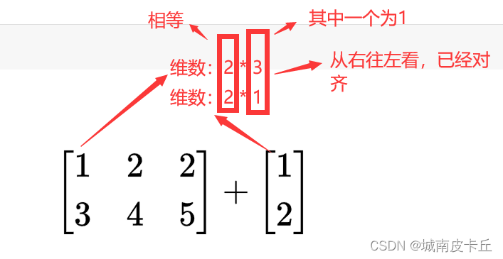
由于pytorch存在的这种广播机制,我们可以对维数不对应的张量进行数学运算,只要这些张量满足以下两个条件:
1.每个张量至少有一个维度
2.满足右对齐
什么是右对齐呢?
下面列举的都为右对齐的情况
情况一:维数不相等(需要从右往左对齐上下,不足的用1补位)上下每一列要么相等,不相等其中一个必须为1
 我们来验证一下张量a,b是否可以进行相加运算
a=torch.rand(2,3,4)
b=torch.rand(3,4)
print(a)
print(a.shape)
print(b)
print(b.shape)
print(a+b)
'''
result:

tensor([[[1.9170e-01, 7.3553e-01, 1.0409e-01, 7.2048e-01],
         [9.9690e-02, 9.8931e-01, 8.0287e-01, 1.6163e-01],
         [2.6184e-01, 1.2664e-01, 3.5558e-01, 7.1151e-01]],

        [[8.2651e-01, 5.7520e-01, 2.5190e-01, 1.5664e-01],
         [4.8740e-01, 3.5411e-01, 4.1564e-01, 4.2516e-04],
         [7.1702e-01, 2.7139e-01, 6.2484e-01, 7.5701e-02]]])
torch.Size([2, 3, 4])
tensor([[0.1759, 0.3124, 0.8845, 0.3470],
        [0.1657, 0.3607, 0.6585, 0.0744],
        [0.4114, 0.1778, 0.6945, 0.9328]])
torch.Size([3, 4])
tensor([[[0.3676, 1.0479, 0.9886, 1.0675],
         [0.2654, 1.3500, 1.4614, 0.2360],
         [0.6733, 0.3045, 1.0501, 1.6443]],
'''
程序没有报错,而且正确输出了结果,验证通过。由于篇幅有限,张量c,d不再验证 。
情况二:维数相等(上下对齐),上下每一列要么相等,若不相等其中一个必须为1
显然我们先前最先验证的例子符合情况二
四、Pytorch中的基本操作
4.1 Pytorch取整、取余相关函数
torch.floor(a) | 将张量a中的每个元素向下取整 |
torch.ceil(a) | 将张量a中的每个元素向上取整 |
torch.round(a) | 将张量a中的每个元素四舍五入 |
torch.trunc(a) | 取张量a中每个元素的整数部分 |
torch.frac(a) | 取张量a中每个元素的小数部分 |
a%2 | 对张量a中的每一个元素对2取余 |
import torch;
'''
pytorch取整、取余相关函数
'''
a=torch.rand(2,2);
a=a*10;
print(a)
print(torch.floor(a))
print(torch.ceil(a))
print(torch.round(a))
print(torch.trunc(a))
print(torch.frac(a))
print(a%2)
tensor([[7.9602, 5.7571],
[5.3785, 0.7960]])
tensor([[7., 5.],
[5., 0.]])
tensor([[8., 6.],
[6., 1.]])
tensor([[8., 6.],
[5., 1.]])
tensor([[7., 5.],
[5., 0.]])
tensor([[0.9602, 0.7571],
[0.3785, 0.7960]])
tensor([[1.9602, 1.7571],
[1.3785, 0.7960]])4.2 pytorch中的三角函数&其他常用函数

 这里的函数非常重要,而且有些函数涉及到深度学习的其他知识,比如激活函数sigmoid。后续单独出章节重点讲解这些函数及其附属知识。这里就不一一像上面逐个举一些简单的例子了
4.3 Pytorch比较运算符
c=torch.rand(2,3)
d=torch.rand(2,3)
print(c)
print(d)
print("eq:")
print(torch.eq(c,d))
print("equal:")
print(torch.equal(c,d))
print("ge:")
print(torch.ge(c,d))
print("gt:")
print(torch.gt(c,d))
print("le:")
print(torch.le(c,d))
print("lt:")
print(torch.lt(c,d))
print("ne:")
print(torch.ne(c,d))
tensor([[0.5555, 0.4367, 0.3116],
[0.5131, 0.1430, 0.9589]])
tensor([[0.3850, 0.0470, 0.5328],
[0.4451, 0.8729, 0.0430]])
eq:
tensor([[False, False, False],
[False, False, False]])
equal:
False
ge:
tensor([[ True, True, False],
[ True, False, True]])
gt:
tensor([[ True, True, False],
[ True, False, True]])
le:
tensor([[False, False, True],
[False, True, False]])
lt:
tensor([[False, False, True],
[False, True, False]])
ne:
tensor([[True, True, True],
[True, True, True]])
4.4 pytorch排序相关函数
f=torch.tensor([1,4,2,6,8])
print(f.shape)
print(torch.sort(f))

#运行结果
'''
torch.Size([5])
torch.return_types.sort(
values=tensor([1, 2, 4, 6, 8]),
indices=tensor([0, 2, 1, 3, 4]))
'''
'''
pytorch排序相关函数
'''
f=torch.tensor([[1,4,2,6,8],
[1,3,5,7,9]])
print(f.shape)
print(torch.sort(f,dim=0,descending=True))
#对于二维数据:dim=0 按列排序,dim=1 按行排序,默认 dim=1
#运行结果
'''
torch.Size([2, 5])
torch.return_types.sort(
values=tensor([[1, 4, 5, 7, 9],
[1, 3, 2, 6, 8]]),
indices=tensor([[0, 0, 1, 1, 1],
[1, 1, 0, 0, 0]]))
'''print(torch.isfinite(f))#判断是否有界
print(torch.isfinite(f/0))
print(torch.isinf(f/0))#判断是否为无穷
print(torch.isnan(f))#判断是不是为空